iterated geodesic triangles

Heisenberg group in Virtual Reality

The Heisenberg group is $\mathbb{R}^3$ with an interesting metric structure. Usually one denotes points in the Heisenberg-Group by $(x,y,t) \in \mathbb{R}^3$. It is an active area of research with many open questions, some for a long time.

This project aims at visualizing and learning about the Heisenberg group in Virtual Reality. The main topics are structure and shapes of geodesics.

This is part of undergraduate research projects in progress with

Celine Cui
Isaiah Glymour
Divya Guwalani
Caroline Kulczycky
Brian Popeck
Matthew Snyder
Amy Waughen
Joshua Ascher

An Introduction to the Heisenberg group

The horizontal space at a point $(x,y,t)$ tells us the permissible directions. Usually it is described as a kernel of a one-form $$ \alpha = dt + 2\left (x\, dy-y\, dx \right ). $$ At a point $(x,y,t)$ the horizontal vectors $v=(v^1,v^2,v^3)$ are exactly those which satisfy $$ 0 = v^3 + 2(x v^2-y v^1) $$ The horizontal vectors form a two-dimensional vector space in $\mathbb{R}^3$ with basis $(X,Y)$ where $$ X := (1, 0, 2y) ,\quad Y:= (0, 1, -2x) $$ and $v = (v^1,v^2,v^3)$ is horizontal if and only if $$ v = v^1 X + v^2 Y $$ The lenght of a (horizontal!) vector $v$ is defined as $\sqrt{|v_1|^2+|v_2|^2}$

A horizontal curve $\gamma: [a,b] \to \mathbb{R}^3$ with derivative $\dot{\gamma}(t)$ satisfies $$ 0=\dot{\gamma}^3(t) + 2(\gamma^1(t)\, \dot{\gamma}^2(t)-\gamma^2(t)\, \dot{\gamma}^1(t)) $$

Observe that this means in particular that if we know the projection into $\mathbb{R}^2$ of $\gamma$, i.e. first two entries of the curve $\gamma^1(t)$ and $\gamma^2(t)$ then we can compute $$ \gamma^3(t) = \gamma^3(0) - \int_0^t 2(\gamma^1(s)\, \dot{\gamma}^2(s)-\gamma^2(s)\, \dot{\gamma}^1(s)) ds $$

The lenght of a (horizontal!) curve is defined as $$ \mathcal{L}(\gamma) := \int_a^b \sqrt{|\dot{\gamma}^1(t)|^2 + |\dot{\gamma}^2(t)|^2}\, dt $$

A curve of (locally) shortest lenght is called a geodesic.

Isometries of the Heisenberg group

There are three ``isometries” for the Heisenberg group:

scaling: for a point $p = (x,y,z)$ and a scale $r > 0$ we define $$\delta_r(p) := (rx,ry,r^2t).$$ If $\gamma: [a,b] \to \mathbb{R}^3$ is a horizontal curve, then so is $\eta(t) := \delta_r \gamma(t)$, and we can compute the lenght $\mathcal{L}(\eta)=r\mathcal{L}(\gamma)$.
translation: this is typically referred to as the group structure: $$ (x,y,t) \ast (x’,y’,t’) := \left (x+x’,y+y’,t+t’+2(x’y-xy’)\right ) $$ If $\gamma: [a,b] \to \mathbb{R}^3$ is a horizontal curve and $p \in \mathbb{R}^3$, then so is $\eta(t) := p \ast \gamma(t)$; The lenght does not change, $\mathcal{L}(\eta)=\mathcal{L}(\gamma)$.
rotations: Let $P$ be a rotation (orientation preserving) in $\mathbb{R}^2$, that is $P \in SO(2)$, or equivalently for some rotation angle $\alpha$ $$ P = \left (\begin{array}{cc}\cos(\alpha) & -\sin(\alpha) \\\sin(\alpha) & \cos(\alpha) \end{array} \right ).$$ We denote by for $v \in \mathbb{R}^3$ let $\tilde{v} = (v^1,v^2)$ be the projection into the $(x,y)$-plane. We then can rotate via $P$ in the $(x,y)$-plane, leaving the $z$-component untouched. $$rot(v,P) := (P\tilde{v},v^3).$$ Let $\gamma: [a,b] \to \mathbb{R}^3$ is a horizontal curve and $P \in SO(2)$ a rotation. Then so is $\eta(t) := rot(\gamma(t),P)$; The lenght does not change, $\mathcal{L}(\eta)=\mathcal{L}(\gamma)$.

Equivalently, for $\alpha \in (0,2\pi)$ and $v \in \mathbb{R}^3$ we have

$$ rot(v,\alpha) := \left (\begin{array}{ccc}\cos(\alpha) & -\sin(\alpha) & 0\\\sin(\alpha) & \cos(\alpha) & 0\\ 0 & 0 & 1\end{array} \right ) v$$

Horizontal straight lines

The simples horizontal lines from a point $p=(p^1,p^2,p^3)$ in the direction of a vector $V \in H_0\mathbb{H}_1$, i.e. $V = (V_1,V_2,0)$ is given by $$ \gamma(t) := p \ast tV=(p^1+tV_1,p^2+tV_2,p^3+2t(V_1 p^2-V_2 p^1)) $$ Indeed then $$ \gamma’(t) = (V_1,V_2,2(V_1 p^2 - V_2 p^1)) $$ which is indeed horizontal at the point $\gamma(t)$ for each $t$.

Computing geodesics of the Heisenberg group

By the isometries for the Heisenberg group we only need to compute geodesics of the following type:

An equivalent metric

The Koranyi-metric on the Heisenberg group for $p=(p_1,p_2,p_3)$ and $q=(q_1,q_2,q_3)$ is given by

$$ (d(p,q)) = \left ( \left (|p_1-q_1|^2+|p_2-q_2|^2\right )^2+|p_3-q_3+2(p_2 q_1-p_1 q_2)|^2 \right )^{\frac{1}{4}}. $$ It is not the same as the Carnot-Caratheodori-metric, but it is equivalent to it.

Now assume we are an object at position $p=(p_1,p_2,p_3)$ wanting to move towards position $q=(q_1,q_2,q_3)$ in a horizontal way, as quickly as possible. If we don’t want to compute the full geodesic (thats expensive), in which direction should we move?

Infimitesimally we can only move in horizontal direction, i.e. we move from $p$ into $p \ast \delta V$ where $V = (V^1,V^2,0)$ – and we want to know how to choose $V$ optimal. We use the method of gradient descent.

Set for $V = (V^1,V^2,0)$ $$ f(V) := (d(p\ast V,q))^4 $$ That is $$ f(V) := |p_1+V^1-q_1|^4+|p_2+V^2-q_2|^4+|p_3-q_3+2(p_2 q_1-p_1 q_2)+2(V^2 q_1-V^1 q_2)|^2 $$ The gradient descent method (analytically this is first order Taylor) tells us that the locally best way to make $f$ smalles is to choose $V$ as $-\delta \nabla f(0)$ for small $\delta>0$.

We have $$ \partial_{V^1} f(0) = 4(p_1-q_1)^3+2(p_3-q_3-4q_2 (p_2 q_1-p_1 q_2)) $$

and $$ \partial_{V^2} f(0) = 4(p_2-q_2)^3+2(p_3-q_3+4q_1 (p_2 q_1-p_1 q_2)) $$ So $$ -\delta \nabla f = -\delta (4(p_1-q_1)^3+2(p_3-q_3-4q_2 (p_2 q_1-p_1 q_2)),4(p_2-q_2)^3+2(p_3-q_3+4q_1 (p_2 q_1-p_1 q_2)),0) $$

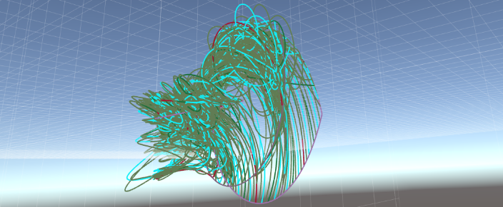
Surface filling with geodesics

It is an open question – often referred to as the Gromov conjecture – how regular a surface embedded into the Heisenberg Group can be. Hajlasz suggested the following method to find a possibly optimal: draw a square with geodesics in the Heisenberg group, then connect midpoints on opposite sides of these squares to fill the square into a surface.

Here are some pictures of how this could look if we do this ``fractal” process for a triangle. In every iteration the midpoints are connected via a geodesic.

Triangle 1