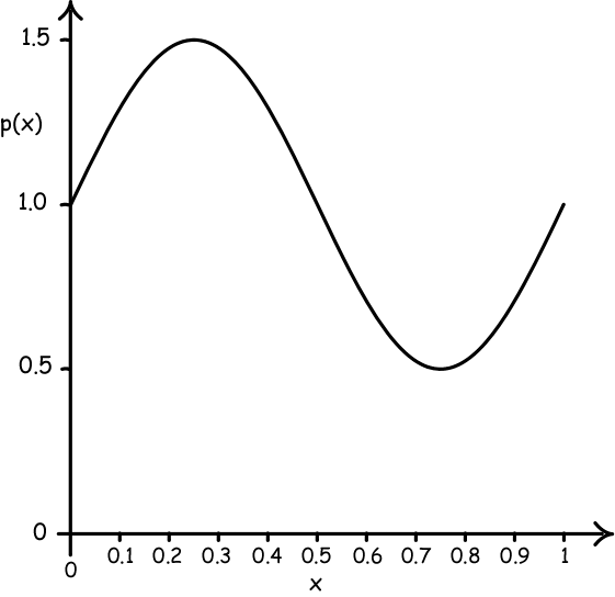
The particular system doesn't really matter. For concreteness, we could imagine that x is the time of year, with x=0 to x=1 spanning an entire year, and the outcome of interest is the time of the day of maximum precipitation.
Since the curve represents a probability density, the probability is given by the area under the curve, which, in total, will be unity.


A continuous probability distribution for x
lies outside the scope of the analysis here. We are considering
finite sets of propositions only. So we need to approximate this
distribution by finite sets of propositions.
To begin, let us consider just two:
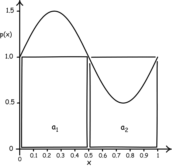
a1 = x lies in (0, 0.5)
a2 = x lies in (0.5, 1)
These are two atoms of a partition that
we will assume to be inductively adapted. As a result, they are
equally probable outcomes. They both have probability 0.5.
P(a1) = P(a2) = 1/2
Areas on the figure opposite measure probability. The two rectangular
areas corresponding to the atoms a1 and a2 are
shown. This partition provides a rather coarse approximation to the
distribution of interest.
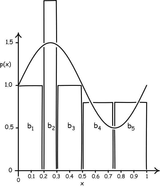
The probability of each atom will be represented by a rectangular area in the figure. That means that range of x values associated with each atoms must vary if the probabilities of the atoms are to come closer to the curve.
For example, the atom associated with the curve's peak must correspond to a narrower range of x values; and the atom associated with the trough must correspond to a wider range of x values.
The refinement displayed opposite is
b1 = x lies in (0, 0.2)
b2 = x lies in (0.2, 0.3)
b3 = x lies in (0.3, 0.5)
b4 = x lies in (0.5, 0.75)
b5 = x lies in (0.75, 1)
What is important for our example is that each of these atoms are equiprobable, so that each has probability 1/5.
As a result, in this new refinement, we have now altered the probability of a2 = (b4 or b5) from its value of 1/2 to
P(a2) = P(b4) + P(b5) = 2/5


What this illustrates is how successive refinements can change the probabilities of the propositions; we have changed the probability of a2 in the last refinement. However as long as the refinements are crafted to approximate the original distribution more and more closely, we can be assured that the probability of a2 will stabilize asymptotically towards the probability assigned by the distribution for outcomes in the range x=0.5 to x=1.
This stabilization is what asymptotic stability requires.
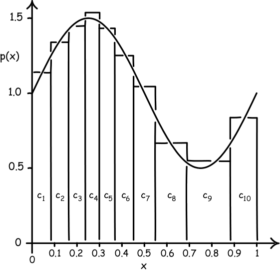
Here is another partition that gives a picture of how close we can
come. This is the partition that arises if we want ten equiprobable
atoms.
The atoms are
c1 = x lies in 0 to 0.09
c2 = x lies in 0.09 to 0.165
c3 = x lies in 0.165 to 0.235
c4 = x lies in 0.235 to 0.300
c5 = x lies in 0.300 to 0.370
c6 = x lies in 0.370 to 0.450
c7 = x lies in 0.450 to 0.545
c8 = x lies in 0.545 to 0.695
c9 = x lies in 0.695 to 0.880
c10 = x lies in 0.880 to 1