| (1) |
In this lab, you will see some applications of the SVD, including
Numerical methods for finding the singular value decomposition
will also be addressed in this lab. One ``obvious''
algorithm involves finding the eigenvalues of ![]() , but this is
not really practical because of roundoff difficulties caused by
squaring the condition number of
, but this is
not really practical because of roundoff difficulties caused by
squaring the condition number of ![]() . Matlab
includes a function called svd with signature
[U S V]=svd(A) to compute the singular value decomposition
and we will be using it, too. This function
uses the Lapack subroutine dgesvd, so if you were to need it in
a Fortran or C program, it would be available by linking against
the Lapack library.
. Matlab
includes a function called svd with signature
[U S V]=svd(A) to compute the singular value decomposition
and we will be using it, too. This function
uses the Lapack subroutine dgesvd, so if you were to need it in
a Fortran or C program, it would be available by linking against
the Lapack library.
You may be interested in a six-minute video made by Cleve Moler in 1976
at what was then known as the Los Alamos Scientific Laboratory. Most
of the film is computer animated graphics. Moler recently retrieved the
film from storage, digitized it, and uploaded it to YouTube at
http://youtu.be/R9UoFyqJca8. You may also be interested in
a description of the making of the film, and its use as background
graphics in the first Star Trek movie, is in his blog at
http://blogs.mathworks.com/cleve/2012/12/10/1976-matrix-singular-value-decomposition-film/
This lab will take three sessions.
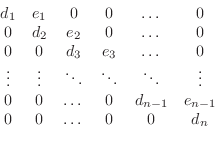
The matrix ![]() in (1) is
in (1) is ![]() and is of the form
and is of the form
and
Supposing that ![]() is the largest integer so that
is the largest integer so that
![]() ,
then the SVD implies that the rank of the matrix is
,
then the SVD implies that the rank of the matrix is ![]() . Similarly,
if the matrix
. Similarly,
if the matrix ![]() is
is ![]() , then the rank of the nullspace
of
, then the rank of the nullspace
of ![]() is
is ![]() . The first
. The first ![]() columns of
columns of ![]() are an orthonormal
basis of the range of
are an orthonormal
basis of the range of ![]() , and the last
, and the last ![]() columns of
columns of ![]() are
an orthonormal basis for the nullspace of
are
an orthonormal basis for the nullspace of ![]() . Of course,
in the presence of roundoff some judgement must be made as to what
constitutes a zero singular value, but the SVD is the best (if
expensive) way to discover the rank and nullity of a matrix.
This is especially
true when there is a large gap between the ``smallest of the large
singular values'' and the ``largest of the small singular values.''
. Of course,
in the presence of roundoff some judgement must be made as to what
constitutes a zero singular value, but the SVD is the best (if
expensive) way to discover the rank and nullity of a matrix.
This is especially
true when there is a large gap between the ``smallest of the large
singular values'' and the ``largest of the small singular values.''
The SVD can also be used to solve a matrix system. Assuming that the matrix is non-singular, all singular values are strictly positive, and the SVD can be used to solve a system.
Further, if
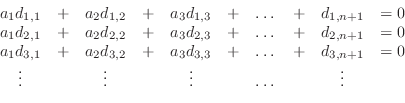
Imagine that you have been given many ``samples'' of related data involving several variables and you wish to find a linear relationship among the variables that approximates the given data in the best-fit sense. This can be written as a rectangular system
The system (3) can be written in matrix form.
Recall that the values ![]() are the unknowns. For a moment, denote
the vector
are the unknowns. For a moment, denote
the vector
![]() , the matrix
, the matrix
![]() and
the vector
and
the vector
![]() , all for
, all for
![]() and
and
![]() , where
, where ![]() .
With this notation, (3) can be written as the
matrix equation
.
With this notation, (3) can be written as the
matrix equation
![]() , where
, where ![]() is (usually)
a rectangular matrix. A ``least-squares'' solution of
is (usually)
a rectangular matrix. A ``least-squares'' solution of
![]() is a vector
is a vector
![]() satisfying
satisfying
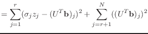
To see why this is so, suppose that the rank of ![]() is
is ![]() , so that there
are precisely
, so that there
are precisely ![]() positive singular values of
positive singular values of ![]() . Then
. Then ![]() and
and
 |
As we have done several times before, we will first generate a data set with known solution and then use svd to recover the known solution. Place Matlab code for the following steps into a script m-file called exer1.m
N=20;
d1=rand(N,1);
d2=rand(N,1);
d3=rand(N,1);
d4=4*d1-3*d2+2*d3-1;
It should be obvious that these vectors satisfy the equation
but, if you were solving a real problem, you would not be aware of this equation, and it would be your objective to discover it, i.e., to find the coefficients in the equation.
EPSILON=1.e-5;
d1=d1.*(1+EPSILON*rand(N,1));
d2=d2.*(1+EPSILON*rand(N,1));
d3=d3.*(1+EPSILON*rand(N,1));
d4=d4.*(1+EPSILON*rand(N,1));
You have now constructed the ``data'' for the following least-squares calculation.
[U S V]=svd(A);Please include the four non-zero values of S in your summary, but not the matrices U and V.
Find this vector by setting b=ones(N,1) (the coefficients in Equation (3) have been moved to the right and are
Sometimes the data you are given turns out to be deficient because the variables supposed to be independent are actually related. This dependency will cause the coefficient matrix to be singular or nearly singular. When the matrix is singular, the system of equations is actually redundant, and one equation can be eliminated. This yields fewer equations than unknowns and any member of an affine subspace can be legitimately regarded as ``the'' solution.
Dealing with dependencies of this sort is one of the greatest difficulties in using least-squares fitting methods because it is hard to know which of the equations is the best one to elminate. The singular value decomposition is the best way to deal with dependencies. In the following exercise you will construct a deficient set of data and see how to use the singular value decomposition to find the solution.
d3=rand(N,1);with the line
d3=d1+d2;This makes the data deficient and introduces nonuniqueness into the solution for the coefficients.
and find the coefficient vector x as in (2). The solution you found is probably not x=[4;-3;2;-1].
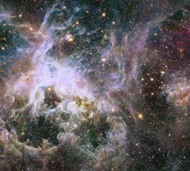
In the following exercise you will see how the singular value decomposition can be used to ``compress'' a graphical figure by representing the figure as a matrix and then using the singular value decomposition to find the closest matrix of lower rank to the original. This approach can form the basis of efficient compression methods.
nasacolor=imread('TarantulaNebula.jpg');
The variable nasacolor will be a
image(nasacolor)
nasa=sum(nasacolor,3,'double');  %sum up red+green+blue
m=max(max(nasa));                %find the max value
nasa=nasa*255/m;                 %make this be bright white
The result from these commands is that nasa is an ordinary
colormap(gray(256));to set a grayscale colormap. Now you can show the picture with the command
image(nasa)
title('Grayscale NASA photo');
Please do not send me this plot.
nasa100=U(:,1:100)*S(1:100,1:100)*V(:,1:100)';
nasa50=U(:,1:50)*S(1:50,1:50)*V(:,1:50)';
nasa25=U(:,1:25)*S(1:25,1:25)*V(:,1:25)';
These matrices are of lower rank than the nasa matrix, and can be stored in a more efficient manner. (The nasa matrix is
We now turn to the question of how to compute the SVD.
The easiest algorithm for SVD is to note the relationship between it
and the eigenvalue decomposition: singular values are the square
roots of the eigenvalues of ![]() or
or ![]() . Indeed, if
. Indeed, if
![]() , then
, then
Unfortunately, this is not a good algorithm because forming the product
![]() roughly squares the condition number, so that the eigenvalue
solution is not likely to be accurate. Of course, it will work fine
for small matrices with small condition numbers and you can
find this algorithm presented in many web pages. Don't believe everything
you see on the internet.
roughly squares the condition number, so that the eigenvalue
solution is not likely to be accurate. Of course, it will work fine
for small matrices with small condition numbers and you can
find this algorithm presented in many web pages. Don't believe everything
you see on the internet.
A more practical algorithm is a Jacobi algorithm that is given in a 1989 report by James Demmel and Krešimir Veselic, that can be found at http://www.netlib.org/lapack/lawnspdf/lawn15.pdf. The algorithm is a one-sided Jacobi iterative algorithm that appears as Algorithm 4.1, p32, of that report. This algorithm amounts to the Jacobi algorithm for finding eigenvalues of a symmetric matrix. (See, for example, J. H. Wilkinson, The Algebraic Eigenvalue Problem, Clarendon Press, Oxford, 1965, or G. H. Golub, C. F. Van Loan, Matrix Computations Johns Hopkins University Press, 3rd Ed, 1996.)
The algorithm implicitly computes the product ![]() and then
uses a sequence of ``Jacobi rotations'' to diagonalize it. A Jacobi
rotation is a
and then
uses a sequence of ``Jacobi rotations'' to diagonalize it. A Jacobi
rotation is a ![]() matrix rotation that annihilates the off-diagonal
term of a symmetric
matrix rotation that annihilates the off-diagonal
term of a symmetric ![]() matrix. You can find more in a nice
Wikipedia article located at
matrix. You can find more in a nice
Wikipedia article located at
http://en.wikipedia.org/wiki/Jacobi_rotation.
Given a ![]() matrix
matrix ![]() with
with
![$\displaystyle M^TM=\left[\begin{array}{cc} \alpha & \gamma \gamma & \beta \end{array}\right]
$](img85.png)
It is possible to find a ``rotation by angle
![$\displaystyle \Theta=\left[\begin{array}{cc} \cos\theta & -\sin\theta
\sin\theta & \cos\theta \end{array}\right]
$](img87.png)
with the property that
where
The following algorithm repeatedly passes down the diagonal of the
implicitly-constructed matrix ![]() , choosing pairs of indices
, choosing pairs of indices ![]() ,
constructing the
,
constructing the ![]() submatrix from the intersection of rows
and columns, and using Jacobi rotations to annhilate the off-diagonal
term. Unfortunately, the Jacobi rotation for the pair
submatrix from the intersection of rows
and columns, and using Jacobi rotations to annhilate the off-diagonal
term. Unfortunately, the Jacobi rotation for the pair ![]() ,
, ![]() messes up the rotation from
messes up the rotation from ![]() ,
, ![]() , so the process must be
repeated until convergence. At convergence, the matrix
, so the process must be
repeated until convergence. At convergence, the matrix ![]() of
the SVD has been implicitly generated, and the right and left singular
vectors are recovered by multiplying all the Jacobi rotations together.
The following algorithm carries out this process.
of
the SVD has been implicitly generated, and the right and left singular
vectors are recovered by multiplying all the Jacobi rotations together.
The following algorithm carries out this process.
Note: For the purpose of this lab, that matrix
![]() will be assumed to be square. Rectangular matrices introduce
too much algorithmic complexity.
will be assumed to be square. Rectangular matrices introduce
too much algorithmic complexity.
Given a convergence criterion ![]() , a square matrix
, a square matrix ![]() ,
a matrix
,
a matrix ![]() , that starts
out as
, that starts
out as ![]() and ends up as a matrix whose columns are left singular
vectors, and another matrix
and ends up as a matrix whose columns are left singular
vectors, and another matrix ![]() that starts out as the identity matrix
and ends up as a matrix whose columns are right singular vectors.
that starts out as the identity matrix
and ends up as a matrix whose columns are right singular vectors.
![$ \left[\begin{array}{cc} \alpha&\gamma \gamma&\beta\end{array}\right]
\equiv$](img100.png) the
the ![$ \left[\begin{array}{cc} \alpha&\gamma \gamma&\beta\end{array}\right]$](img106.png) )
)
function [U,S,V]=jacobi_svd(A)
% [U S V]=jacobi_svd(A)
% A is original square matrix
% Singular values come back in S (diag matrix)
% orig matrix = U*S*V'
%
% One-sided Jacobi algorithm for SVD
% lawn15: Demmel, Veselic, 1989,
% Algorithm 4.1, p. 32

TOL=1.e-8;
MAX_STEPS=40;

n=size(A,1);
U=A;
V=eye(n);
for steps=1:MAX_STEPS
  converge=0;
  for j=2:n
    for k=1:j-1
      % compute [alpha gamma;gamma beta]=(k,j) submatrix of U'*U
      alpha=???  %might be more than 1 line
      beta=???   %might be more than 1 line
      gamma=???  %might be more than 1 line
      converge=max(converge,abs(gamma)/sqrt(alpha*beta));

      % compute Jacobi rotation that diagonalizes
      %    [alpha gamma;gamma beta]
      if gamma ~= 0
        zeta=(beta-alpha)/(2*gamma);
        t=sign(zeta)/(abs(zeta)+sqrt(1+zeta^2));
      else
        % if gamma=0, then zeta=infinity and t=0
        t=0;
      end
      c=???
      s=???

      % update columns k and j of U
      T=U(:,k);
      U(:,k)=c*T-s*U(:,j);
      U(:,j)=s*T+c*U(:,j);

      % update matrix V of right singular vectors

      ???

    end
  end
  if converge < TOL
    break;
  end
end
if steps >= MAX_STEPS
  error('jacobi_svd failed to converge!');
end

% the singular values are the norms of the columns of U
% the left singular vectors are the normalized columns of U
for j=1:n
  singvals(j)=norm(U(:,j));
  U(:,j)=U(:,j)/singvals(j);
end
S=diag(singvals);
U=[0.6  0.8
   0.8 -0.6];
V=sqrt(2)/2*[1  1
             1 -1];
S=diag([5 4]);
It is easy to see that U and V are orthogonal matrices,
so that the matrices U, S and V comprise the
SVD of A. You may get a ``division by zero'' error, but this
is harmless because it comes from gamma being zero, which
will cause zeta to be infinite and t to be zero
anyhow.
Your algorithm should essentially reproduce the matrices U, S and V. You might find that the diagonal entries of S are not in order, so that the U and V are similarly permuted, or you might observe that certain columns of U or V have been multiplied by (-1). Be sure, however, that an even number of factors of (-1) have been introduced.
If you do not get the right answers, you can debug your code in the following way. First, note that there is only a single term, k=1 and j=2 in the double for loop.
A1 = [ 1  3  2
       5  6  4
       7  8  9];
Check that U1 and V1 are orthogonal matrices
and that A1=U1*S1*V1' up to roundoff. In addition,
print U1, S1 and V1 using format long
and visually compare them with the singular values you get from the Matlab
svd function. You should find they agree almost to roundoff,
despite the coarse tolerance inside jacobi_svd. You also
will note that the values do not come out sorted, as they do from
svd. It is a simple matter to sort them, but then you
would have to permute the columns of U1 and V1 to
match. Again, some columns of U1 and V1 might
be multiplied by (-1) and, if so, there must be an even number of
those sign changes. Please include U1, S1 and V1
in your summary.
You now have an implementation of one SVD algorithm. This algorithm is a good one, with some realistic applications, and is one of the two algorithms available for the SVD in the GNU scientific library. (See http://www.gnu.org/software/gsl/ for more detail.) In the following sections, you will see a different algorithm.
The most commonly used SVD algorithm is found in Matlab and in the Lapack linear algebra library. (See http://www.netlib.org/lapack/.) It is a revised version of one that appeared in Golub and Van Loan. The revised version is presented by J. Demmel, W. Kahan, ``Accurate Singular Values of Bidiagonal Matrices,'' SIAM J. Sci. Stat. Comput., 11(1990) pp. 873-912. This paper can also be found at http://www.netlib.org/lapack/lawnspdf/lawn03.pdf.
The standard algorithm is a two-step algorithm. It first reduces the matrix to bidiagonal form and then finds the SVD of the bidiagonal matrix. Reduction to bidiagonal form is accomplished using Householder transformations, a topic you have already seen. Finding the SVD of a bidiagonal matrix is an iterative process that must be carefully performed in order to minimize both numerical errors and the number of iterations required. To accomplish these tasks, the algorithm chooses whether Golub and Van Loan's original algorithm is better than Demmel and Kahan's, or vice-versa. Further, other choices are made to speed up each iteration. There is not time to discuss all these details, so we will only consider a simplified version of Demmel and Kahan's zero-shift algorithm.
In the Jacobi algorithm in the previous section, you saw how the two
matrices ![]() and
and ![]() can be constructed by multiplying the various
rotation matrices as the iterations progress. This procedure is the
same for the standard algorithm, so, in the interest of simplicity,
most of the rest of this lab will be concerned only with the singular
values themselves.
can be constructed by multiplying the various
rotation matrices as the iterations progress. This procedure is the
same for the standard algorithm, so, in the interest of simplicity,
most of the rest of this lab will be concerned only with the singular
values themselves.
The first step in the algorithm is to reduce the matrix to bidiagonal
form. You have already seen how to use Householder matrices to
reduce a matrix to upper-triangular form. The idea, you recall,
is to start with matrices ![]() and
and ![]() equal to the identity matrix
and
equal to the identity matrix
and ![]() , so that
, so that
![]() . Then,
. Then,
function [U,B,V]=bidiag_reduction(A)
% [U B V]=bidiag_reduction(A)
% Algorithm 6.5-1 in Golub & Van Loan, Matrix Computations
% Johns Hopkins University Press
% Finds an upper bidiagonal matrix B so that A=U*B*V'
% with U,V orthogonal.  A is an m x n matrix

[m,n]=size(A);
B=A;
U=eye(m);
V=eye(n);
for k=1:n-1
  % eliminate non-zeros below the diagonal
  % Keep the product U*B unchanged
  H=householder(B(:,k),k);
  B=H*B;
  U=U*H';

  % eliminate non-zeros to the right of the
  % superdiagonal by working with the transpose
  % Keep the product B*V' unchanged

  ???

end
A=rand(100,100);Be sure that the condition that A=U*B*V' is satisfied, that the matrix B is bidiagonal, and that U and V are orthogonal matrices. Describe how you checked these facts and include the results of your tests in the summary. Hint: You can use the Matlab diag function to extract any diagonal from a matrix or to reconstruct a matrix from a diagonal. Use ``help diag'' to find out how. Alternatively, you can use the tril and triu functions.
An important piece of Demmel and Kahan's algorithm is a very efficient
way of generating a ![]() ``Givens'' rotation matrix that annihilates
the second component of a vector. The algorithm is presented
on page 13 of their paper and is called ``rot.'' It is important to have
an efficient algorithm because this step is the central step in
computing the SVD. A 10% (for example) reduction in time for
rot translates into a 10% reduction in time for the SVD.
``Givens'' rotation matrix that annihilates
the second component of a vector. The algorithm is presented
on page 13 of their paper and is called ``rot.'' It is important to have
an efficient algorithm because this step is the central step in
computing the SVD. A 10% (for example) reduction in time for
rot translates into a 10% reduction in time for the SVD.
This algorithm computes the cosine, ![]() , and sine,
, and sine, ![]() , of a rotation
angle that satisfies the following condition.
, of a rotation
angle that satisfies the following condition.
![$\displaystyle \left[\begin{array}{cc} c & s -s & c\end{array}\right]
\left[\b...
...ay}{c} f g\end{array}\right]=
\left[\begin{array}{c} r 0\end{array}\right]
$](img136.png)
Remark: The two different expressions for ![]() ,
, ![]() and
and ![]() are mathematically equivalent. The choice of which to do is based on
minimizing roundoff errors.
are mathematically equivalent. The choice of which to do is based on
minimizing roundoff errors.
function [c,s,r]=rot(f,g)
% [c s r]=rot(f,g)
% more comments

% your name and the date
[c s;-s c]*[f;g]and check that the resulting vector is [r;0].
[c s;-s c]*[f;g]and check that the resulting vector is [r;0].
[c s;-s c]*[f;g]and check that the resulting vector is [r;0].
The standard algorithm is based on repeated QR-type ``sweeps'' through
the bidiagonal matrix. Suppose ![]() is a bidiagonal matrix, so
that it looks like the following.
is a bidiagonal matrix, so
that it looks like the following.
In its simplest form, a sweep begins at the top left of the matrix and
runs down the rows to the bottom. For row ![]() , the sweep first
annihilates the
, the sweep first
annihilates the ![]() entry by multiplying on the right by a rotation
matrix. This action introduces a non-zero value
entry by multiplying on the right by a rotation
matrix. This action introduces a non-zero value ![]() immediately below the diagonal. This new non-zero is then
annihilated by multiplying on the left by a rotation matrix but this
action introduces a non-zero value
immediately below the diagonal. This new non-zero is then
annihilated by multiplying on the left by a rotation matrix but this
action introduces a non-zero value ![]() , outside the upper
diagonal, but the next row down. Conveniently, this new non-zero is
annihilated by the same rotation matrix that annihilates
, outside the upper
diagonal, but the next row down. Conveniently, this new non-zero is
annihilated by the same rotation matrix that annihilates ![]() .
(The proof uses the fact that
.
(The proof uses the fact that ![]() was zero as a
consequence of the first rotation, see the paper.) The algorithm
continues until the final step on the bottom row that introduces no
non-zeros. This process has been termed ``chasing the bulge'' and
will be illustrated in the following exercise.
was zero as a
consequence of the first rotation, see the paper.) The algorithm
continues until the final step on the bottom row that introduces no
non-zeros. This process has been termed ``chasing the bulge'' and
will be illustrated in the following exercise.
The following Matlab code implements the above algorithm. This code will be used in the following exercise to illustrate the algorithm.
function B=msweep(B)
% B=msweep(B)
% Demmel & Kahan zero-shift QR downward sweep
% B starts as a bidiagonal matrix and is returned as
% a bidiagonal matrix

n=size(B,1);
for k=1:n-1
  [c s r]=rot(B(k,k),B(k,k+1));

  % Construct matrix Q and multiply on the right by Q'.
  % Q annihilates both B(k-1,k+1) and B(k,k+1)
  % but makes B(k+1,k) non-zero.
  Q=eye(n);
  Q(k:k+1,k:k+1)=[c s;-s c];
  B=B*Q';

  [c s r]=rot(B(k,k),B(k+1,k));

  % Construct matrix Q and multiply on the left by Q.
  % Q annihilates B(k+1,k) but makes B(k,k+1) and
  % B(k,k+2) non-zero.
  Q=eye(n);
  Q(k:k+1,k:k+1)=[c s;-s c];
  B=Q*B;

end
In this algorithm, there are two orthogonal (rotation) matrices, ![]() ,
employed. To see what their action is, consider the piece of
,
employed. To see what their action is, consider the piece of
![]() consisting of rows and columns
consisting of rows and columns ![]() ,
, ![]() ,
, ![]() , and
, and ![]() .
Multiplying on the right by the transpose of the first rotation matrix
has the following consequence.
.
Multiplying on the right by the transpose of the first rotation matrix
has the following consequence.
![$\displaystyle \left[\begin{array}{cccc}\alpha& * &\beta&0\\
0 & * & * & 0\\
...
...0\\
0 & * & 0 & 0\\
0 & * & * & *\\
0 & 0 & 0 & \gamma\end{array}\right]
$](img162.png)
where asterisks indicate (possible) non-zeros and Greek letters indicate values that do not change. The fact that two entries are annihilated in the third column is not obvious and is proved in the paper.
The second matrix ![]() multiplies on the left and has the following consequence.
multiplies on the left and has the following consequence.
![$\displaystyle \left[\begin{array}{cccc} 1 & 0 & 0 & 0\\
0 & c & s & 0\\
0 &...
...0\\
0 & * & * & *\\
0 & 0 & * & *\\
0 & 0 & 0 & \gamma\end{array}\right]
$](img163.png)
The important consequence of these two rotations is that the row with three non-zeros in it (the ``bulge'') has moved from row
  % set almost-zero entries to true zero
  % display matrix and wait for a key
  B(find(abs(B)<1.e-13))=0;
  spy(B)
  disp('Plot completed. Strike a key to continue.')
  pause
Insert two copies of this code into msweep.m, one
after each of the statements that start off ``B=.''
B=[1 11  0  0  0  0  0  0  0  0
   0  2 12  0  0  0  0  0  0  0
   0  0  3 13  0  0  0  0  0  0
   0  0  0  4 14  0  0  0  0  0
   0  0  0  0  5 15  0  0  0  0
   0  0  0  0  0  6 16  0  0  0
   0  0  0  0  0  0  7 17  0  0
   0  0  0  0  0  0  0  8 18  0
   0  0  0  0  0  0  0  0  9 19
   0  0  0  0  0  0  0  0  0 10];
The sequence of plots shows the ``bulge'' (extra non-zero entry) migrates from the top of the matrix down the rows until it disappears off the end. Please include any one of the plots with your work. If B=msweep(B); what is B(10,10)?
Demmel and Kahan present a streamlined form of this algorithm in their paper. This algorithm is not only faster but is more accurate because there are no subtractions to introduce cancellation and roundoff inaccuracy. Their algorithm is presented below.
The largest difference in speed comes from the representation of
the bidiagonal matrix ![]() as a pair of vectors,
as a pair of vectors, ![]() and
and ![]() , the
diagonal and superdiagonal entries, respectively. In addition,
the intermediate product,
, the
diagonal and superdiagonal entries, respectively. In addition,
the intermediate product, ![]() , is not explicitly formed.
, is not explicitly formed.
This algorithm begins and ends with the two vectors ![]() and
and ![]() ,
representing the diagonal and superdiagonal of a bidiagonal matrix.
The vector
,
representing the diagonal and superdiagonal of a bidiagonal matrix.
The vector ![]() has length
has length ![]() .
.
function [d,e]=vsweep(d,e)
% [d e]=vsweep(d,e)
% comments

% your name and the date
B=[1 11  0  0  0  0  0  0  0  0
   0  2 12  0  0  0  0  0  0  0
   0  0  3 13  0  0  0  0  0  0
   0  0  0  4 14  0  0  0  0  0
   0  0  0  0  5 15  0  0  0  0
   0  0  0  0  0  6 16  0  0  0
   0  0  0  0  0  0  7 17  0  0
   0  0  0  0  0  0  0  8 18  0
   0  0  0  0  0  0  0  0  9 19
   0  0  0  0  0  0  0  0  0 10];
d=diag(B);
e=diag(B,1);
n=200;
d=2*rand(n,1)-1; %random numbers between -1 and 1
e=2*rand(n-1,1)-1;
B=diag(d)+diag(e,1);
tic;B=msweep(B);mtime=toc
tic;[d e]=vsweep(d,e);vtime=toc
norm(d-diag(B))
norm(e-diag(B,1))
It turns out that repeated sweeps tend to reduce the size of the
superdiagonal entries. You can find a discussion of convergence
in Demmel and Kahan, and the references therein, but the basic
idea is to watch the values of ![]() and when they become small,
set them to zero. Demmel and Kahan prove that this does not perturb
the singular values much. In the following exercise, you will see
how the superdiagonal size decreases.
and when they become small,
set them to zero. Demmel and Kahan prove that this does not perturb
the singular values much. In the following exercise, you will see
how the superdiagonal size decreases.
d=[1;2;3;4;5;6;7;8;9;10];
e=[11;12;13;14;15;16;17;18;19];
Use the following code to plot the absolute values
for k=1:15
  [d,e]=vsweep(d,e);
  plot(abs(e),'*-')
  hold on
  disp('Strike a key to continue.')
  pause
end
hold off
starting from the values of e and d above.
You should observe that some
entries converge quite rapidly to zero, and they all eventually decrease.
Please include this plot with your summary.
d=[1;2;3;4;5;6;7;8;9;10];
e=[11;12;13;14;15;16;17;18;19];
Please include this plot with your summary.
You should have observed that one entry converges very rapidly to zero, and that overall convergence to zero is asymptotically linear. It is often one of the two ends that converges most rapidly. Further, a judiciously chosen shift can make convergence even more rapid. We will not investigate these issues further here, but you can be sure that the software appearing, for example, in Lapack (used by Matlab) for the SVD takes advantage of these and other acceleration methods.
In the following exercise, the superdiagonal is examined during the iteration. As the values become small, they are set to zero, and the iteration continues with a smaller matrix. When all the superdiagonals are zero, the iteration is complete.
function [d,iterations]=bd_svd(d,e)
% [d,iterations]=bd_svd(d,e)
% more comments

% your name and the date

TOL=100*eps;
n=length(d);
maxit=500*n^2;

% The following convergence criterion is discussed by
% Demmel and Kahan.
lambda(n)=abs(d(n));
for j=n-1:-1:1
  lambda(j)=abs(d(j))*lambda(j+1)/(lambda(j+1)+abs(e(j)));
end
mu(1)=abs(d(1));
for j=1:n-1
  mu(j+1)=abs(d(j+1))*mu(j)/(mu(j)+abs(e(j)));
end
sigmaLower=min(min(lambda),min(mu));
thresh=max(TOL*sigmaLower,maxit*realmin);


iUpper=n-1;
iLower=1;
for iterations=1:maxit
  % reduce problem size when some zeros are
  % on the superdiagonal

  % Don't iterate further if value e values are small
  % how many small values are near the bottom right?
  j=iUpper;
  for i=iUpper:-1:1
    if abs(e(i))>thresh
      j=i;
      break;
    end
  end
  iUpper=j;
  % how many small values are near the top left?
  j=iUpper;
  for i=iLower:iUpper
    if abs(e(i))>thresh
      j=i;
      break;
    end
  end
  iLower=j;

  if (iUpper==iLower & abs(e(iUpper))<=thresh) | ...
        (iUpper<iLower)
    % all done, sort singular values
    d=sort(abs(d),1,'descend');  %change to descending sort
    return
  end

  % do a sweep
  [d(iLower:iUpper+1),e(iLower:iUpper)]= ...
        vsweep(d(iLower:iUpper+1),e(iLower:iUpper));
end
error('bd_svd: too many iterations!')
d=[1;2;3;4;5;6;7;8;9;10];
e=[11;12;13;14;15;16;17;18;19];
B=diag(d)+diag(e,1);
What are the singular values that bd_svd produces? How many iterations did bd_svd need? What is the largest of the differences between the singular values bd_svd found and those that the Matlab function svd found for the matrix B?
d=rand(30,1);
e=rand(29,1);
B=diag(d)+diag(e,1);
Use bd_svd to compute its singular values. How many iterations does it take? What is the largest of the differences between the singular values bd_svd found and those that the Matlab function svd found for the matrix B?
Remark: In the above algorithm, you can see that
the singular values are forced to be positive by taking absolute
values. This is legal because if a negative singular value arises
then multiplying both it and the corresponding column of ![]() by
negative one does not change the unitary nature of
by
negative one does not change the unitary nature of ![]() and leaves
the singular value positive.
and leaves
the singular value positive.
You saw in the previous exercise that the number of iterations can get large. It turns out that the number of iterations is dramatically reduced by the proper choice of shift, and tricks such as sometimes choosing to run sweeps up from the bottom right to the top left instead of always down as we did, depending on the matrix elements. Nonetheless, the presentation here should give you the flavor of the algorithm used.
In the following exercise, you will put your two functions, bidiag_reduction and bd_svd together into a function mysvd to find the singular values of a full matrix.
function [d,iterations]=mysvd(A)
% [d,iterations]=mysvd(A)
% more comments

% your name and the date
This function should:
``Latent semantic indexing'' is a very interesting idea that uses
SVD to help index natural
language documents. One explanation that is more complete
than the one here can be found in the Wikipedia:
http://en.wikipedia.org/wiki/Latent_semantic_analysis.
Suppose you are given a number of documents and
a number (not the same number) of words that appear in some or all
of the documents. First, create an ``incidence matrix'' that has
a 1 in position ![]() if the
if the
![]() th
document contains at
least one occurrance of the
th
document contains at
least one occurrance of the
![]() th
word, and 0 otherwise.
th
word, and 0 otherwise.
It is important to realize that if you are given ![]() words and
construct a vector with a 1 in positions corresponding to the given
words, then multiplying the incidence matrix by this vector will yield
a vector
words and
construct a vector with a 1 in positions corresponding to the given
words, then multiplying the incidence matrix by this vector will yield
a vector
![]() with entries
with entries
![]() and with the
and with the
![]() indicating how many of the given words appear in the
indicating how many of the given words appear in the
![]() th
document.
th
document.
It is natural, then to compute the SVD of the incidence matrix
and keep only the singular vectors with large singular values, just
as was done earlier in compressing the Mars picture. The SVD
comes with a bonus: the right singular vectors (the columns of
![]() ) provide groupings of words that are related according to
their use in the documents, and can be regarded as ``concepts''
appearing in the documents. The left singular vectors (the
columns of
) provide groupings of words that are related according to
their use in the documents, and can be regarded as ``concepts''
appearing in the documents. The left singular vectors (the
columns of ![]() ) provide groupings of the documents according
to the words. The most surprising of the features of the SVD
is that multiplication of the incidence matrix by a vector
representing a group of words will identify precisely those documents
containing the words but a similar multiplication by the matrix
constructed of only a few singular values will identify documents
containing related words!
) provide groupings of the documents according
to the words. The most surprising of the features of the SVD
is that multiplication of the incidence matrix by a vector
representing a group of words will identify precisely those documents
containing the words but a similar multiplication by the matrix
constructed of only a few singular values will identify documents
containing related words!
In the following exercise, you will see an example of this process from which you can draw your own conclusions.
To generate the exercise, I took a list of titles of publications from the Math Department web site a few years ago and extracted a list of words and constructed an incidence matrix from the titles (regarded as ``documents'') and the words. You will see how the SVD is able to identify ``concepts'' consisting of groups of words related because of the way they are used in the titles. You will also see how one could use the SVD to identify documents that employ certain words.
I must mention a caveat. This example is flawed by its use of titles and authors from departmental research reports. In the first place, the number of titles is not large, and in the second place, the titles themselves are too short to clearly elicit relationships among words. Titles and authors are used because it was convenient to gather the data and because you students might be familiar with the authors and topics. A better choice would have been the abstracts of the articles instead of their titles, but these were not conveniently available.
Results in the following exercise can be better understood if you are aware of various specialized groups of Mathematics faculty. For example, the Mathematics Department web pages describe the Mathematical Biology group as consisting of Professors Doiron, Ermentrout, Rubin, Swigon, and Troy, and the Numerical Analysis and Scientific Computing group as consisting of Professors Layton, Neilan, Trenchea, and Yotov. Prof. Neilan joined the faculty after the list of publications used in this exercise was constructed.
Before continuing, you need to understand how a new Matlab data structure is used. It is called a ``cell array'' and you can think of it as an array of cells in a spreadsheet. The contents of the cells can be just about anything and in this case will be strings of varying lengths. An ordinary Matlab array of strings would have to have all strings of the same length-not a convenient way to store titles of papers.
A cell array is indicated by ``braces'' or ``curly brackets'': ``{'' and ``}''. An ordinary column vector of numbers might be defined
v=[1;2;3;4;5];while a cell array containing strings would be defined using curly brackets as
c={'one';'second string';'third';'4';'the fifth string is long.'}
There are two ways to refer to the contents of a cell array.
Cell arrays can contain any Matlab data in their cells. A cell array might have a string in its first position, a matrix in its second position, a vector in its third position, and another cell array in its fourth position. This flexibility provides great power to the script writer, but we will only be using cell arrays that contain strings of varying lengths, and the reason we are using cell arrays and not string arrays is because a cell array can contain strings of varying lengths while a string array can contain only strings of the same lengths.
For the following exercise, I have constructed three cell arrays and a matrix, and they are included in the file reports_data.m.
c={'one';'second string';'third';'4';'the fifth string is long.'}
Please answer the following questions.
ss = 'The cascade of Brinkman code';use word_vec to construct a vector, v, corresponding to the words appearing in ss. How many of the distinguished words appear in ss? Check that v is correct with the following commands.
words{find(v==1)}
Be sure that the words printed are the ones appearing in ss.
C = U(:,1:25) * S(1:25,1:25) * V(:,1:25)' ;
t = C * v;
where v is the vector associated with the single word ``canard,'' will yield a selection of titles satisfying the criterion abs(t) > 0.2. Please include the list of titles in your summary. It is interesting that one of the titles containing the word ``canard'' itself does not appear in this list but that all the titles refer to behavior of excited synapses in neurons, from which one could conclude that the word ``canard'' refers to the behavior of excited synapses under certain circumstances.
Back to MATH2071 page.