Growth in Multifactor Productivity

indicates that an economy can increase output per worker or q by

1. increasing the amount of capital per worker or k. See the previous web page for a study of growth by capital accumulation.
2. increasing multifactor productivity or A. An increase in A will come from innovation in methods of production, due to improved technology or improved organization -- including improved transportation and infrastructure under technology, and a decrease in social friction under organization.

To understand the approach, consider the Solow model presented earlier:

As we saw, this model would result in a steady-state output of 2500 and a steady-state capital stock of 625 if growth were due exclusively to capital accumulation.

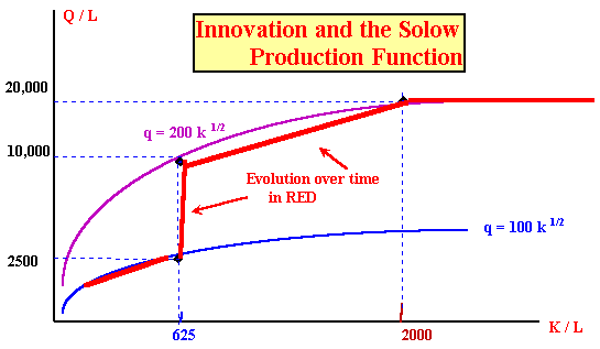
The simplest way to model an innovation is to have the model's multifactor productivity coefficient increase from 100 to 200. With a capital stock of 625, this means that output would increase from 2500 to 5000.

This would not be the end of the story, however: the innovation would give rise to more investment -- an increase in productivity will mean a higher steady state level of capital and of output. We may calculate the new steady-state by using:

1. the new production function:
   q = 200 k ^0.5

2. the savings function:
   s = 0.25 q

3. the equilibrium condition:
   s = k

   savings must replace capital stock.

Substitute the new production function into this equation to get:

or (dividing by k ^0.5

or, squaring both sides,

The equilibrium capital stock increased from 625 to 2500; equilibrium output will increase From 2500 to 10,000.

Note that although the increase in multifactor productivity is directly responsible for only a doubling of production, without the increase in productivity the capital stock would not have increased from 625 to 2500 -- and indirectly the increase in multifactor productivity is responsible for the entire increase in output.

Graphical presentation

In the diagram below, we trace the time path of the economy, assuming that the economy grows along the old production function until it reaches a steady state of 625 units of capital and 2500 units of output, that an innovation occurs which instantaneously increases output to 5000 by changing the production function to q = 200 k ^0.5 and that the economy then grows along the new production function until it reaches its new steady state output of 10,000.

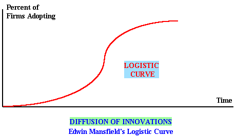
One further step in the direction of realism is to make the impact of the innovation take time rather than be reflected in an instantaneous jump. We know a good deal about the way in which innovations are introduced in specific industries, thanks to the works of Edwin Mansfield (US, University of Pennsylvania). In a series of studies on specific industries, from steel to beer bottling, Mansfield found that the transition to a new technique, as measured by the fraction of the firms adopting the technique, invariably followed a logistic curve . The typical logistic curve is illustrated below:

A moment's thought shows that this is quite logical: the first innovators will find the job a difficult one, later innovators will find things very easy, and the last to adopt the innovation will find not much to do and equally importantly not much in the way of profits to be made since they are facing stiff competition from firms already in place. The first railroads had to pay the costs of experimentation, later railroads benefitted from the efforts of the pioneers, and the last railroads duplicated existing services.

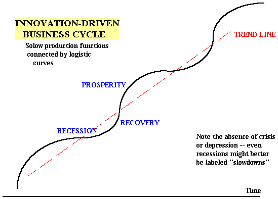
If we put several logistic curves together as transitions from one production function to another, we should see how it was possible for Schumpeter to maintain that innovation alone can generate business cycles:

If cycles come from innovation, then they are an essential feature of capitalist economic development. They cannot be eliminated without also eliminating innovation; Schumpeter concluded that we should not be too quick to intervene to smooth out the business cycle. Even failures and bankruptcies were -- in part at least -- a necessary "creative destruction" of old industries and a clearing of the ground for new industries. Only the slowing down of profits from old ways of doing things provides the incentive to innovate; keeping the profits of blacksmiths high gives them no incentive to shift to automobile manufacturing.

However, as Schumpeter also admitted, the business cycle often went farther than necessary in the process of boom and depression. Note in the diagram above that we have periods of recovery, prosperity and "recession" or slower than average growth -- but that the recessions do not involve declines in output, merely a period of slow growth. If this were all there was to the macroeconomic story, it would be a relatively happy one. However, the more accurate picture of the macroeconomy involves both booms or periods of faster than warranted growth and depressions or periods of contraction of output .

Note: Schumpeter's distinction between recessions and depressions is a logical one which perhaps should have been adopted; however, reluctance to use the term "depression" has led economists to distinguish "growth recessions" in which output continues to grow, but at a slower than average pace from "recessions" in which output falls for two quarters in a row -- and to avoid the nasty term "depression" entirely.

In looking for the cause of depressions and booms, the two principal suspects are:

1. monetary events -- excess credit creation by banks and excess money issue by the central government can lead to a temporary boom, but not to long term growth, and in fact will typically lead to inflation and then a reaction against inflation which may well plunge the economy into depression.
2. errors of expectation -- which may lead to excess optimism by businesses in their investment plans or consumers in their purchasing (especially on installment credit, if they expect future income to be steadily increasing).

How to recognize and control that excess variability are the central problems of macroeconomics.