(1)
where rand() is a uniformly distributed random number on the interval (0,1).
XPPAUT is a program I wrote for the simulation of dynamical systems. Since equation (1) is just an iteration, it is easy to use XPP to simulate it. By convention, files that XPP uses have the extension ode . Here is the code for poisson.ode
# the simple Poisson process
dt=-log(ran(1))/rate
tfire'=tfire+dt
aux isi=dt
par rate=.05
@ bound=200000,total=4000,meth=discrete
done
Type
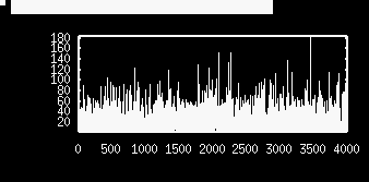
xppaut poisson.odeto run XPP on this file. Note that the rate is 0.05 which is in milliseconds and corresponds to 50 Hz. You can find various tutorials on XPP on my web page here . Click on Initialconds Go . Click on Xivst and choose isi as the variable to plot. You will see a nice set of interspike intervals

which looks alot like random noise. Now
we will compute the coefficient of variation by taking the ratio of
the mean and the standard deviation. Click on nUmerics stocHastic
Stat Mean and choose isi as the variable. In a second
it should return with something like
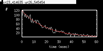
Click on OK to dismiss the window. We are still in the Numerics menu, so lets make a histogram of the ISI's. Click on stocHastic Histogram and set bins=100, lo=0, hi=60, variable=isi and just hit return for the condition. Click on Escape to go back to the main menu and then click on Xivst and choose tfire as the variable to plot. XPP always puts the histogram in the first two columns. You will see a nice histogram. I have also plotted the function 120 exp(-0.05 t) alongside to show how well the simulation matches the exponential distribution.
The simulation above computes 4000 spikes no matter what. So, how could we run this simulation so that it stops after a fixed amount of time? The variable tfire tracks the current time of the spike. So we should just stop the simulation when tfire=1000 and then see how many iterates that we ran. This is the number of spikes in 1000 msec. If we do this over say, 1000 trials, we can compute the Fano factor. You can make XPP stop when tfire=1000 and from this obtain the number of iterates that it took. This is the spike count. Because of the way XPP computes stopping points, the iteration at which it stops is interpolated between two times so we have to take the integer part of the count. Click on Numerics Poincare map Section and fill it in like
| Variable | TFIRE |
| Section: | 1000 |
| Direction (+1,-1,0): | 1 |
| Stop on sect(y/n): | Y |
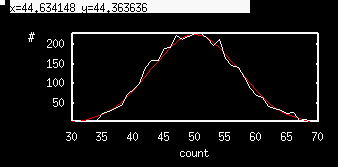
Then click Ok You have told XPP to stop when tfire =1000 . Click Escape and then Initconds Go . If you look in the Data Viewer you will see a single row and the first entry in the row is the count. It is in the Time column since "Time" to XPP means iteration number. Integrate the equations again and you will get a different number. Do this many times and you will see that the counts are centered around 50. Lets average 1000 trials. XPP lets you repeat iterations many times using the Initconds Range command. This produces a dialog box which you should fill in as follows:
| Range Over: | tfire |
| Steps | 1000 |
| Start: | 0 |
| End: | 0 |
| Reset storage (Y/N): | N |
Ignore the other entries and click Ok After a moment, it will
be done and the Time column will be filled with the spike
counts for each of the 1000 trials. Note that these should be
truncated. Since the error encountered by not truncating them is
small, we don't need to. (However, if you want, click on Replace
in the Data Viewer and choose
t to replace. Then for the formula type in flr(t)
which takes the integer part.) Now take the mean and standard
deviation by clicking nUmerics stocHastic Stat Mean and
choose t as the variable. I got
# poisson process with refractory
# period
# s0=0 for no refractory
r=rmax*(1-s0*s)
# define a two-step Markov process with rate r
markov z 2
{0} {r}
{1} {0}
# define a flag so that when z jumps past 1/2
# reset it to 0, turn on refractory period and
# increment the count
global 1 z-.5 {s=1;z=0;count=count+1}
# exponential decay of the refractory period
s'=-s/tau
count'=0
par rmax=.05,tau=10,s0=0
@ meth=euler,dt=.1,total=1000,bound=1000000,nout=500,trans=1000
done
I have added comments to perhaps explain what is going on here. I only keep the last data point which contains the count at the end of 1000 msec. Basically, the z variable flips to 1 at a rate r . When z crosses the value .5 then several events are flagged:
For the first set of experiments, we are only interested in the spike count for a trial of 1 second (1000 msec). Run this and integrate it a few times looking at the last row in the Data Viewer to see the count. It should be between 40 and 60 since we initially do not use the the refractory period. ( s0=0 so that there is no dependence of r on the variable s . Now we will check this method to see that it leads to a Fano factor of about 1 as predicted. We want to repeat this simulation for 500 trials to get a list of spike counts. Click on Initconds Range and fill in the dialog box as:
| Range Over: | s |
| Steps | 500 |
| Start: | 0 |
| End: | 0 |
| Reset storage (Y/N): | N |
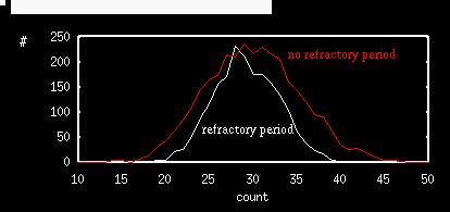
and ignore the other entries and then press OK. After a bit (not too much) the simulation will end and you will have a spike count list for 500 trials. Click on nUmerics stocHastic Stat Mean and choose count as the variable. A window will pop with the mean and the standard deviation. I got mean=50.12 and std.dev.=7.03 which gives a Fano factor of .986, pretty close to the theoretical value of 1. Note that mean is 50 which is the predicted value. Escape back to the main menu. In the Parameter window change s0=1. Click on Initconds Range and click on Ok since the dialog is filled as we want. After the simulation, find the mean and the standard deviation for the spike count. I got mean=35.5, std.dev=4.25 so the spike count is considerably lower. The Fano factor is about 0.5. Try the simulation a few more times to see that this is not a fluke. Try tau=5,15,20 and increase the number if trials to 2000 (change the 500 steps to 2000 in the above dialog box). (This may take a bit of time; it took me a minute and a half.) Below I show the spike count histogram for no refractory period and 600 msec trials along with that of a 20 msec refractory period and 1000 msec trials. Note the clear difference in the widths of the distributions. Refractory periods tend to regularize the distribution.
We can use the same file to compute the ISI distribution for a long single trial with and without the refractory period. To do this, we will plot the times between the event of the variable s jumping to 1 (indicating a spike). Here is how to set it up. Get the numerics menu: click on nUmerics . Now
| Variable | s |
| Section: | .993 |
| Direction (+1,-1,0): | 1 |
| Stop on sect(y/n): | N |
This tells XPP to look for whenever s crosses 0.993. Then it computes the time between this event and the last time it occurred. This is the "period" between events, the ISI. It stores this in the "time" column.
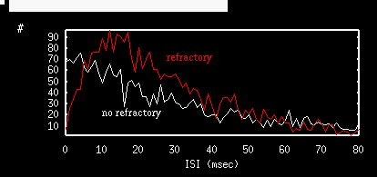
Repeat these experiments with different values of the refractory period and see how the CV is also decreased.
# poisper.ode
# inhomogeneous process
markov z 2
{0} {r}
{100} {0}
# rate is periodic
r=.02+.025*cos(.01*pi*t)
# check for events and output when event occurs
global 1 z-.5 {out_put=1}
# numerical stuff and storage issues
#
@ meth=euler,dt=.1,maxstor=500000,total=30000,trans=40000
# keep track of the stimulus for testin
aux stim=r
done
Run XPP and click on Initiconds Go. This will generate the spike times. Now click on nUmerics stocHastic Autocorrelation choose 2000 for the number of bins, -1000 for Low, 1000 for Hi, and T for the variable. Escape to the main menu and click Xivst choosing Z and you will get the autocorrelogram.