Stochastic Models of Channels

At the microscopic level, channels are stochastic event with probabities of turning on and off. With the advent of patch clamping and other experimental procedures, it is possible to record from a single channel while stepping through many different voltages. Here I will look at some simple and then more complex models. First, let's consider for example the potassium channel for the Morris-Lecar model. The current for this is:

I_K = g n (V - E_K)

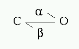
The gate n just satisfies the first order kinetic scheme:

The rates are voltage dependent. However, for a fixed value of the voltage, they are fixed. We simulate the stochastic process as follows. We choose a time step, dt and choose a random number, r between 0 and 1. If we are in the closed state C and alpha dt > r then we jump to the open state. Otherwise, we stay at the closed state. Similarly, if we are in the open state O and beta dt > r then we jump to the closed state.

For the Morris -Lecar equation, we are given only tau and ninf so that we obtain:

alpha = ninf/tau

beta = (1-ninf)/tau

XPP has a built-in routine to handle random switching called the Markov object. For an n-state system, you define an n dimensional square matrix. The entries of row j contain the rates of transition from state j to any other state k . The diagonals are set to zero since they are really just the probabilities of staying where you are so given the other entries, these diagonals are determined.

Simulate the Morris-Lecar channel given the kinetics:

ninf(v) = (1+tanh((v-12)/17.4)/2

tau(v) = 1/(phi cosh((v-12)/34.8))

where the rate constant phi=.0666 and you step from -100 mV to 0 mV for a total of 60 msec. Integrate this a bunch of times and eventually you will see a channel opening. If you want to just run it, click here for an XPP file. If you are lucky, you may see a single channel opening since this is a real slow channel. Change the rate constant to make it much faster, say, 1 and run To see how this approaches the deterministic limit, you could simulate 10 or 100 such channels and look at the sum. But since all the channels are independent, you could, instead, just repeat the simulation for one channel many times and do a trial average. To do this in XPP, just click on nUmerics stochastics Compute and fill in the dialog box as follows:

Range Over:	z
Steps	100
Start:	0
End:	0

and press OK to repeat the simulation 100 times. XPP keeps track of the mean and variance over the trials at each time point. When complete, click on stocHastic Mean and then on Esc to get to the main menu. Click on Restore to see a rough approximation of the deterministic limit.

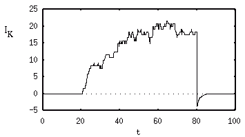
Even as few as 100 channels is pretty damn close to the deterministic limit. The law of mass action is pretty awesome. Note the little negative blip occuring after the stimulus. This is because the channels take some time to turn off and the potential has been brought back to -100 mV which is below the equilibrium potential for potassium.

Hodgkin-Huxley channels

The potassium and sodium channels for the HH equations are more complicated. Recall the HH potassium current is given by:

I_K = g n⁴(V-E_K)

One can consider the channel as having 5 states: 0000, 0001, 0011, 0111, 1111 where only yhe last state is conducting. Here is a kinetic model for the channel:

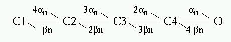
with C1=0000 and O = 1111 being the completely closed and open states respectively. We can use the standard HH kinetics for potassium to simulate a voltage clamp with a holding potential of -100 mV and then a step to +20 mV for 20 milliseconds. The following XPP file implements a stochastic simulation of this channel using a 5 state markov process with the rates defined by the usual HH equations. Try integrating this a few times. Look at the mean after 10 trials (equivalent to 10 channels) and 100 trials. It looks pretty much like the ML. Note that the channel is much faster and thus looks much more like the mean field equations over the time course of 20 msec.

The sodium channel is more complicated. The following kinetic scheme becaomes the standard HH sodium model in the mean field limit:

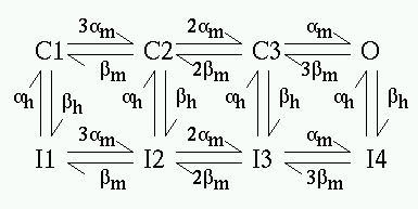
which is an EIGHT!! state model. In the last 15 years, more careful experiments shed doubt on this model and Patlak has devised a more realistic model for this which has the following kinetic scheme:

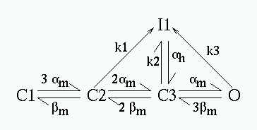
The transitions to the inactive state I1 are all voltage independent and can occur from three different points in the system. The alpha's and beta's are all as in the standard HH model and the remaining parameters are k1=0.24, k2=0.4, k3=1.5 all in msec^-1. You should simulate this for a 20 msec step from -100 mV to 20 mV and look at the sodium current which is

I_Na = g O (V-E_Na)

Here is an XPP file if you don't want to try it yourself. The result of a simulation of 1, 10, and 100 channels (trials) is shown here:

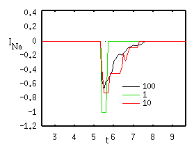
Note that the current is scaled and has no particular units.

Homework

Write down and simulate a single channel model for the Morris-Lecar calcium channel
Write down a kinetic scheme for the T-type calcium channel assuming the the channel has the following current:

I_T = g m² h (V-E_ca)
(Hint: it will look alot like the 8 state sodium channel but with fewer states.)
Simulate a three-state model which has the following transitions:
- closed -> open 10/sec
- open -> closed 100/sec
- open -> inactive 50/sec
- inactive -> open 5/sec
You should take 0.5 msec time steps. What is the faction of time it is in the open state? Can you figure this out analytically? (Hint: the steady state distribution is related to the eigenvalues of the transition matrix.)