Lesson 1

In this tutorial, you will learn to write a very simple ode file for the logistic equation:

To write an ODE file, just follow these simple steps:

1. Click on on the far right of the menu bar at the top to create a new ODE.
2. The text editor will pop up. In the file name box, type in the name first.ode
3. Delete the text in the textbox that says Type ODE..... XPP uses x' to denote the derivative and requires the file end with done Type the following

   x'=x*(1-x)
   done
   

4. That's it! You have written your first ODE file. Now let's run it.

   Click Save to save it.

   XPP has many defaults; among them is that all initial conditions are set to zero.

5. If the file is OK, and you haven't made some mistakes, like forgetting the *, then the main menu will appear.

   If you have made a mistake, XPP, will tell you and will bring up the logfile . This file may give you some info on why the file failed.

6. Click in the top menu bar to solve and plot the ODE. You won't see much there since the solution is x(t)=0.
7. You can change the initial conditions in two ways for this file
   • Click on the button and change 0 to, say, 0.1 and then tap outside the menu. Click again to see a less trivial trajectory.
   • What is even cooler is to use the sliders.
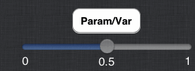
     1. Click on one of the parameter sliders
     2. Choose X with the scroll wheel
     3. Edit the minimum value to -1
     4. Tap outside the window
     5. Now move the slider and watch the solutions evolve
8. That's it. Not much left to do with this ODE

Lesson 2 - planar ODE

1. Open the editor for a new file by tapping
2. Call the ODE second.ode and clear the Type ODE... part
3. Type in the following

   # second.ode
   x'=x*(1-a*x-b*y)
   y'=y*(-c+d*x)
   par a=1,b=1,c=0.5,d=1
   init x=1,y=.1
   done
   

   There are three new parts to the ODE file. The # indicates a comment and is ignored by XPP. You can put comments wherever you want. Another new feature is the declaration of parameters. You must tell XPP about parameters that are in the problem. Parameters are always declared as name=value with the value being a number. IMPORTANT Do not put spaces around the = sign in the parameter declaration! The last new feature is the init declaration which sets the initial values. As with parameters, it is always of the form name=value . Of course, you can change the parameters and the initial conditions once the ODE file is loaded.
4. Save and if there are no errors, the ODE. ( If there are errors, look at the log file and fix them. )
5. Let's change the view from X vs t to a phaseplane.
   • Touch the screen with two fingers. This brings up the graphics dialog.
   • Change xlo=-0.1,xhi=1.1,ylo=-.1,yhi=1.1 and move the wheels so that X is on the x-axis and Y is on the y-axis. You will see the plot change as in the image below. Press Done
   • Now you have a phaseplane view
6. Press and hold to bring up a dialog and tap Direction fields This draws direction fields.
7. Press and hold and choose Nullclines to get the nullclines
8. Tap in the phaseplane to integrate with a new initial condition
9. Tap on to freeze the curves as you tap. Press and hold and choose Integrate Backwards to solve backwards in time
10. Tap to clear the graphs
11. Tap on a slider and pick c as the parameter and let the range go from 0 to 2
12. Tap on a different slider and choose a with a range of 0 to 2 also.
13. Move the sliders and watch the nullclines, direction field, and trajectory change on the fly.
14. Intersections of the nullclines are equilibria. Press and hold near an intersection and choose Equilibrium from point and XPP will tell you what type of equilibrium it is. If there is one positive eigenvalue or one negative eigenvalue, XPP will automatically compute and draw the unstable or stable manifolds.
15. Manually change parameters by tapping

Howto's

1. Click on to change the numerics
   • Choose the integration method. For discrete dynamical systems choose DISCRETE
   • The rest are numerical parameters
2. Export data In XPP, click on the on top and the data from the run will be saved as odename.ode.dat You can then get it by the same way that you add Tables (see next item).
3. Tables If you want to load a table into the iPad version of XPP, you have to put the table in a place where it can be found.
   • When the iPad is attached to your computer, click on the iPad in iTunes
   • Open the APP tab and scroll all the way down to the File Sharing section
   • Scroll down to XPP and click on it.
   • Click on tha Add button and then choose the table. You can also use this to add more ODE files and to delete them
4. Range integration Since the GUI doesn't yet support things like Poincare maps and range integration, you can use the internal options to set these up within the ODE file. in particular, to automatically run a range integration, add @ range=1 to your ODE. Look at logbif.ode to see an example of this sort of thing
5. Boundary value problems If you have set up your ODE to have boundary conditions, you can tap to edit the BCs and tap to run it. Since the sliders only call the initial value solver, you can force XPP to use the BVP solver as follows
   • In the ODE file, add the parameter line

     par ibvp=0
     

   • In XPP, change IBVP=1 to run the BVP solver and IBBV=0 to run the initial value solver
6. Averaging and adjoints Add the line par ibvp=0 to your ODE file. Compute exactly one period of a limit cycle. You will probably have to adjust Total the total integration time. Set IBVP=2 and press to get the adjoint. To compute the interaction function, open the window and put the right-hand sides in the available entries. Tap anywher to close the window. Set IBVP=3 and then tap to get the H function.
7. Where is AUTO? It's an iPad dude