Teaching · Phys 3274
Computational Physics
Modern computational methods open up a realm of physics that pencil and paper cannot reach: complex, nonlinear phenomena, from chaos to phase transitions.
1About the course
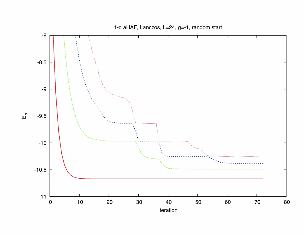
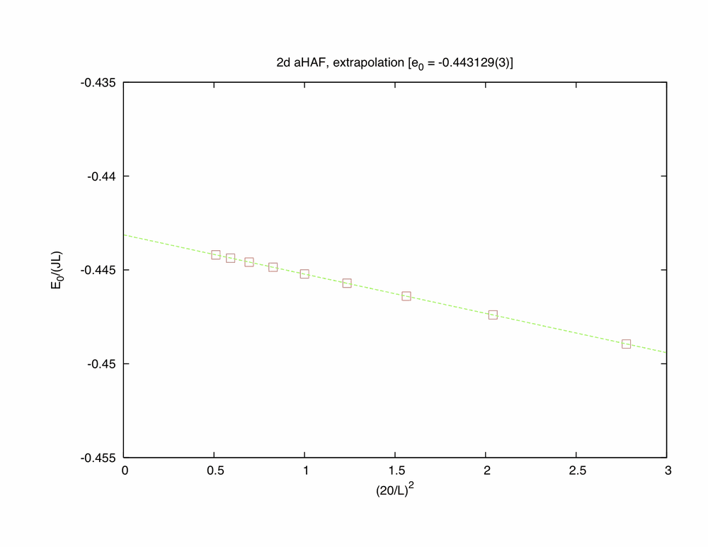
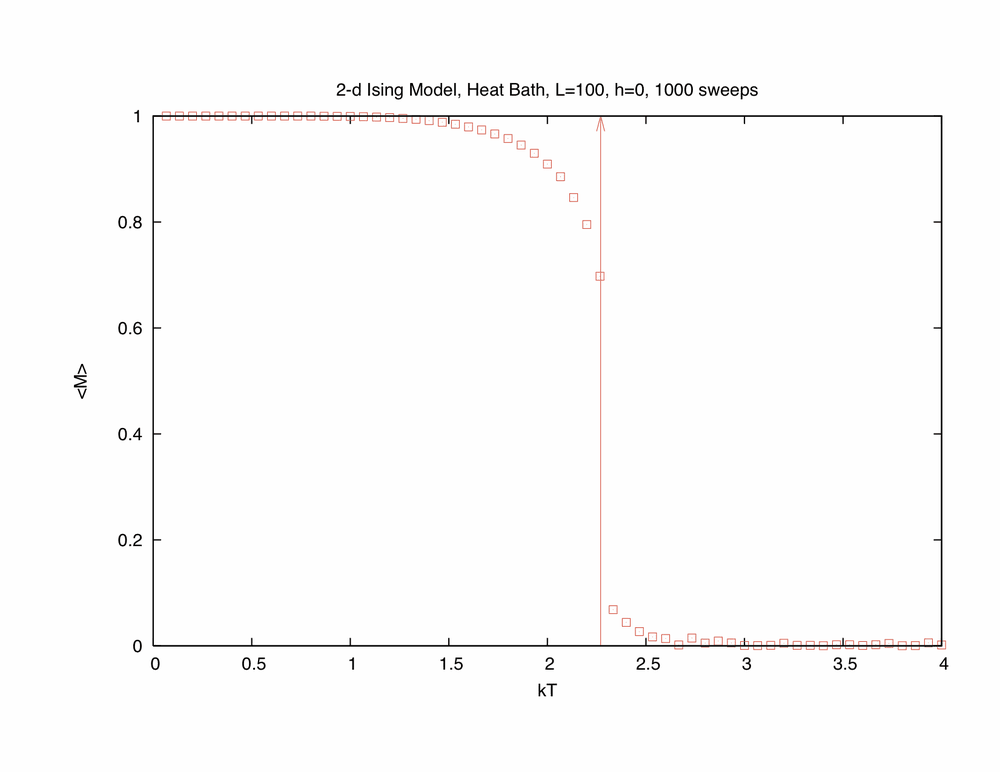
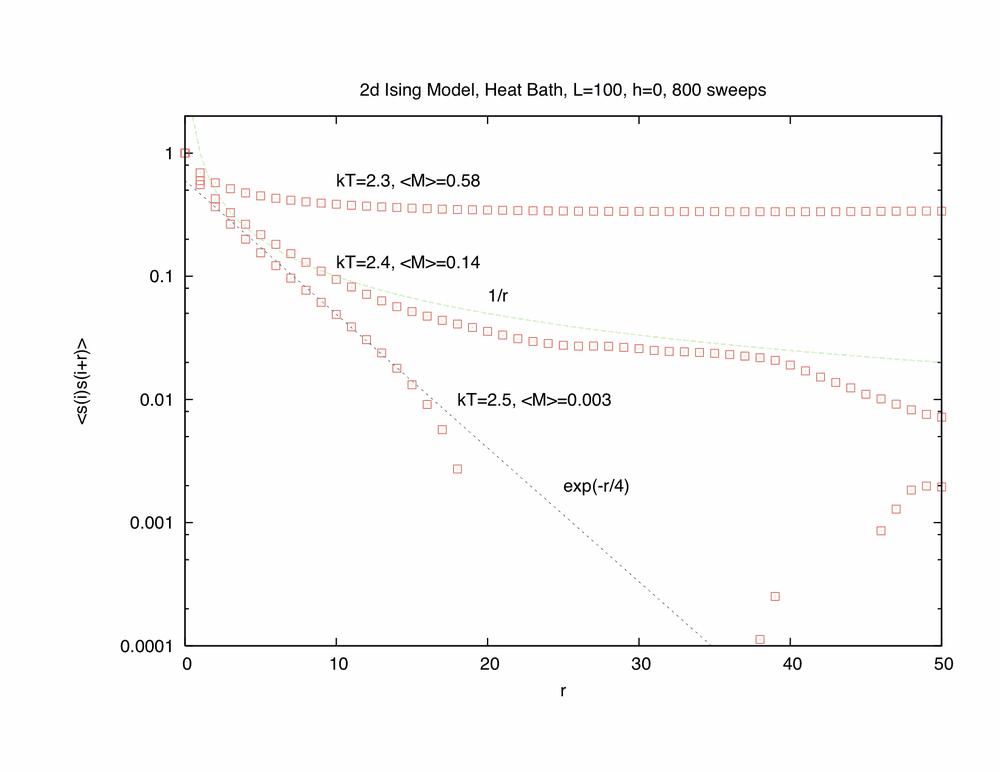
The course explores classic examples of what computation makes possible: the logistic map, nonlinear oscillators, chaotic planetary motion, molecular dynamics and the Ising model. Along the way it covers the working tools: coding, numerical integration, differential equations, quantum scattering and bound states, quantum magnetism, and the Monte Carlo method for classical and quantum systems.
The focus is on physics. No prior computing experience is required, but students are expected to learn a programming language if they do not know one already, and the learning curve is steep. The aim is a computer-literate graduate student who knows what computers can do, where to find the resources, and how to produce and present research of professional quality.
By the end of the course students are able to
- assess whether a complex physics problem can be solved computationally;
- design an efficient approach to solving it;
- locate the resources that make a solution possible;
- produce publication-quality graphs and written reports.
2Topics
- Coding basics
- Arrays, matrices, loops, input and output, graphing, programming style, testing and debugging, understanding the problem.
- Numbers
- Binary representation, floating-point precision, the largest and smallest numbers, errors and stability.
- Integration, differentiation and extrapolation
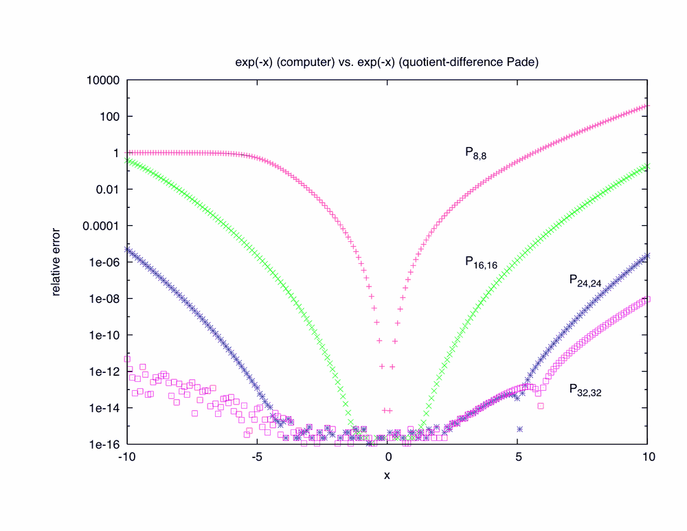
- Discretisation, evaluating polynomials, continued fractions, Borel summation, Padé approximants, extrapolation and interpolation, quadrature (including singular integrands and adaptive methods), simple Monte Carlo, Fourier transforms and the FFT.
- Ordinary differential equations
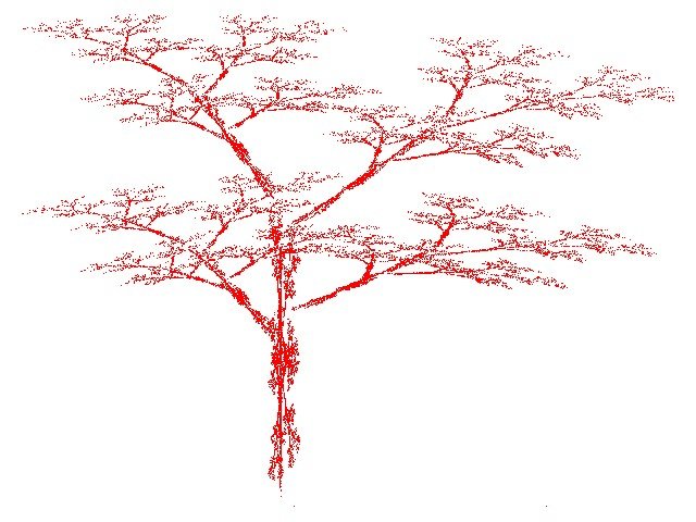
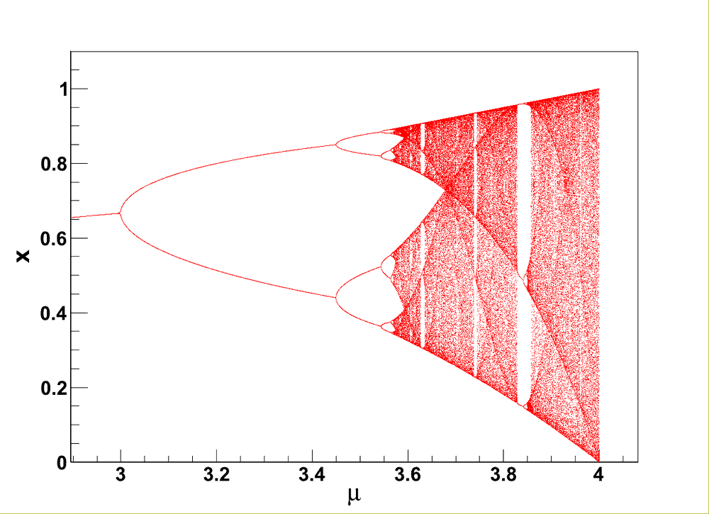
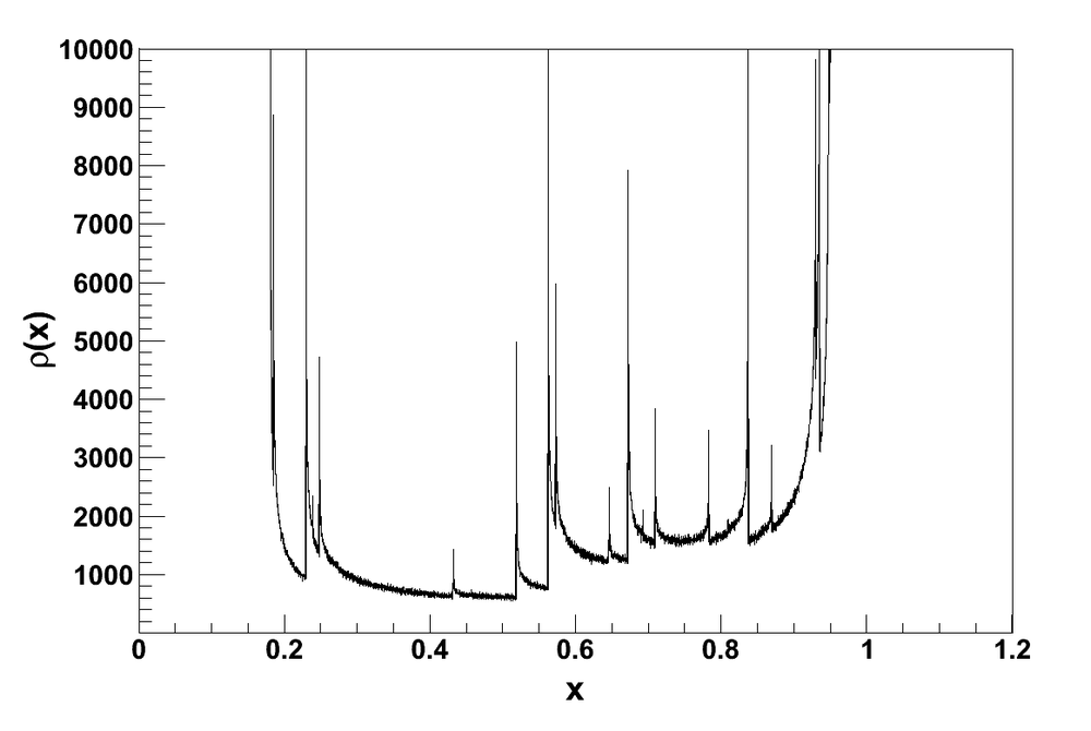
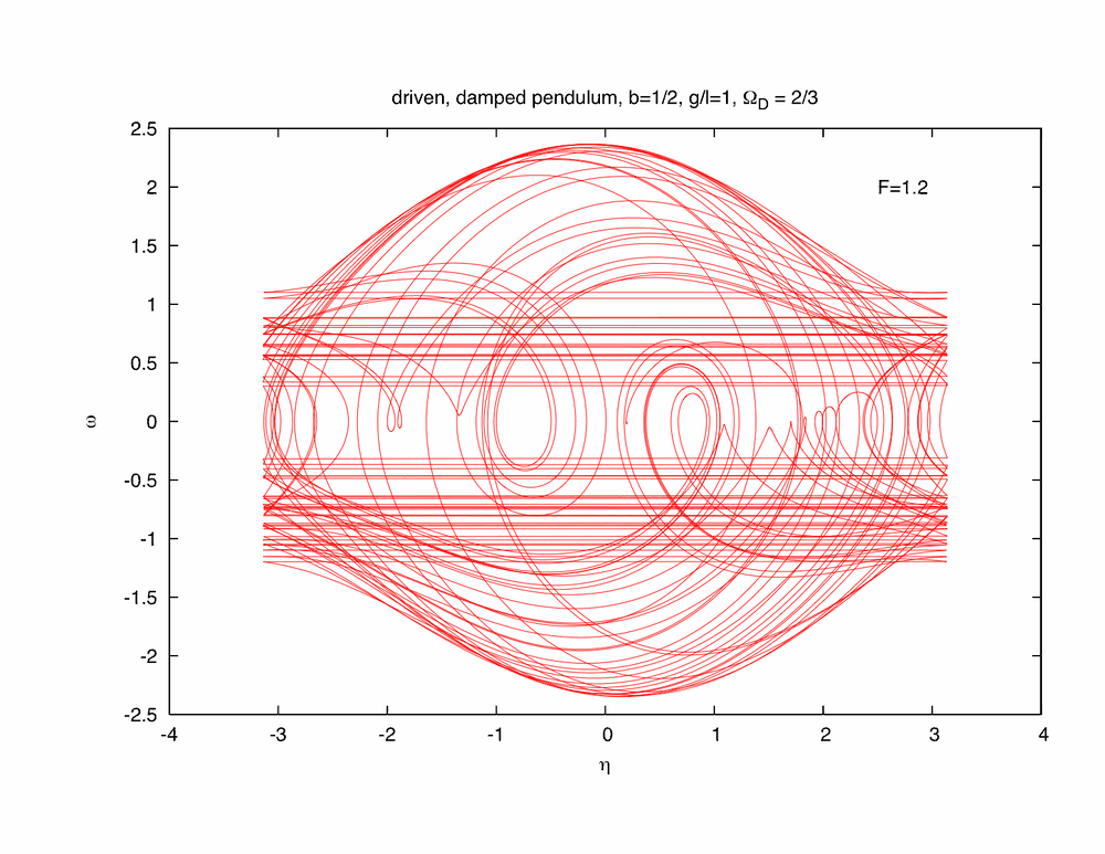
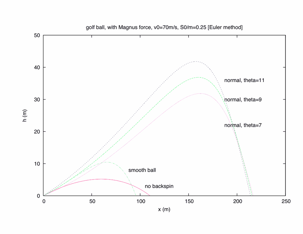
- Differencing, Euler, Euler–Cromer and Runge–Kutta methods; the damped, driven oscillator; chaos; the logistic map; fractal plants.
- Partial differential equations
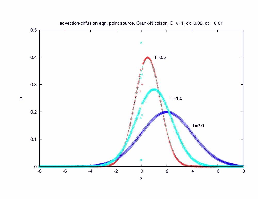
- Relaxation and multigrid methods, error analysis and stability, explicit and implicit schemes, the advection–diffusion problem.
- Molecular dynamics
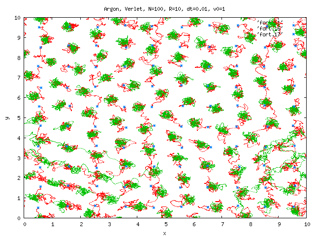
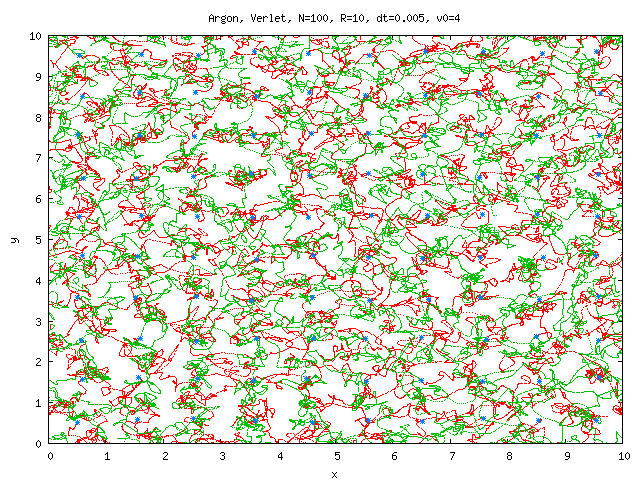
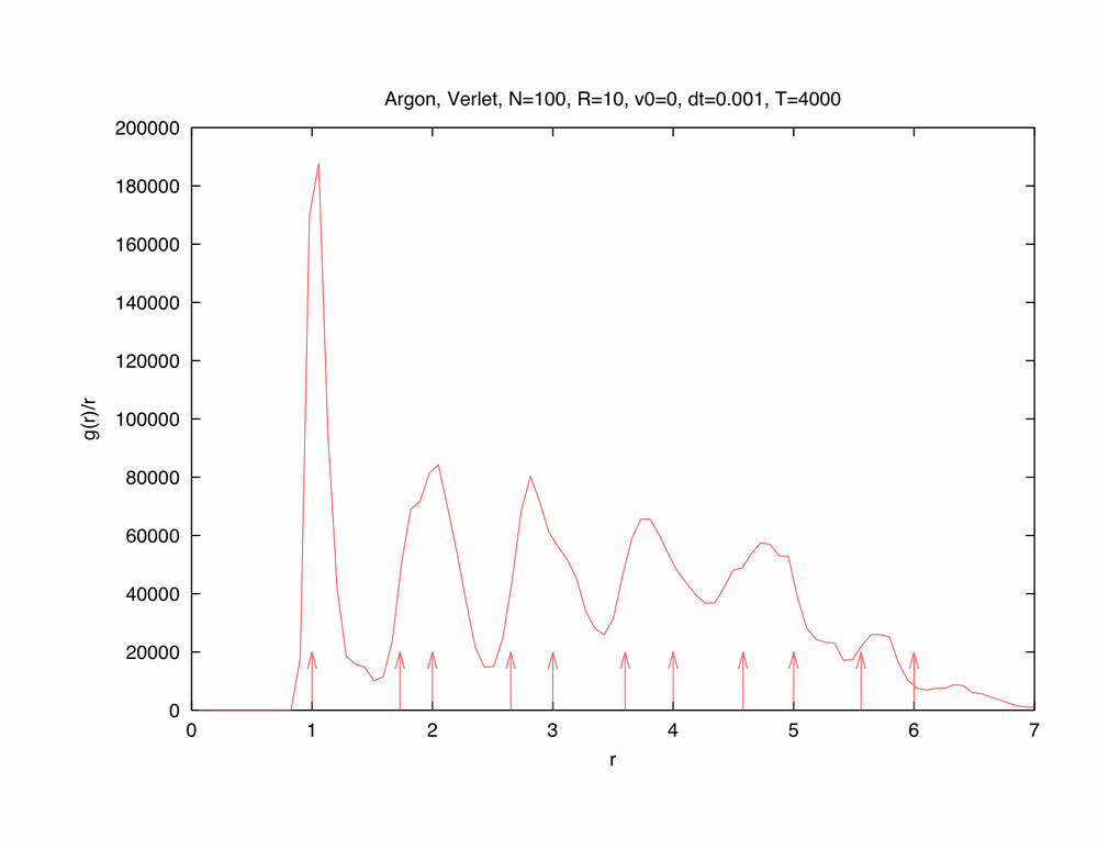
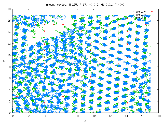
- Gases, the equipartition theorem, melting, the Fermi–Pasta–Ulam problem.
- Linear algebra and quantum mechanics
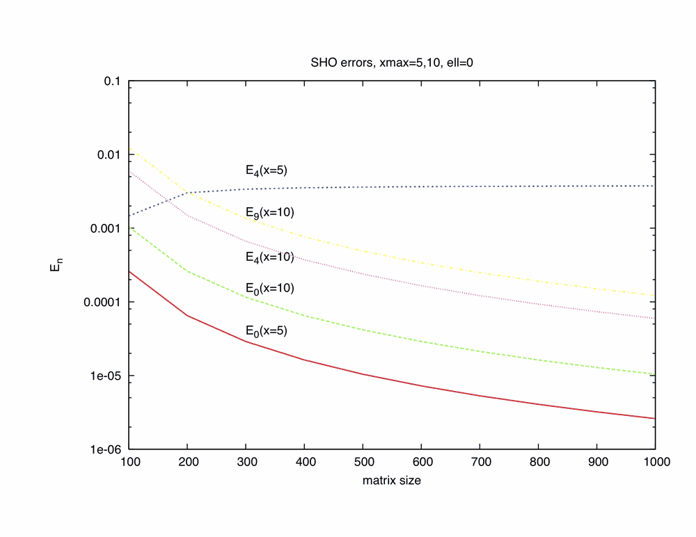
- Matrix inversion and integral equations; diagonalisation, tridiagonal systems and the Lanczos algorithm; the one-dimensional Schrödinger equation in a basis, bound states, and scattering in momentum space (the T-matrix); minimisation and fitting.
- The Monte Carlo method
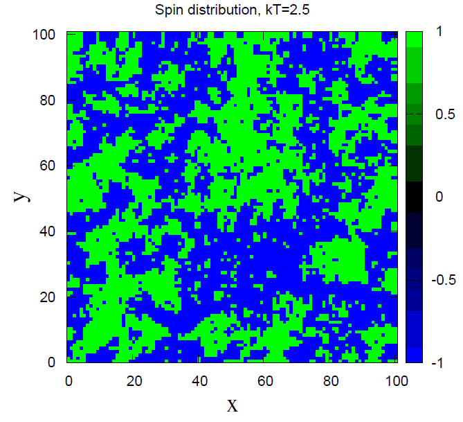
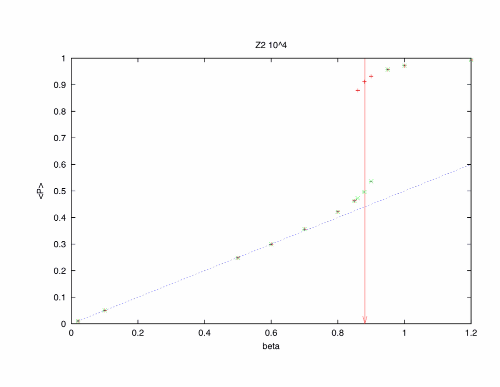
- Random numbers, Markov chains, ergodicity, the Metropolis and heat-bath algorithms, annealing; applications to percolation, the Ising model and Z(2) lattice gauge theory.
- Computational physics today
- A survey, with the emphasis on algorithms: lattice gauge theory, climate modelling, numerical relativity, supernovae, protein folding, quantum spin systems, nuclear physics.
3Images from the course
Results from the course work. Click an image to see it full size.
Chaos and dynamical systems
Numerics and differential equations
Molecular dynamics
Quantum magnetism
Monte Carlo
4Books
Text: J. F. Boudreau and E. S. Swanson, Applied Computational Physics, Oxford University Press (2018).
Also useful:
- W. H. Press, S. A. Teukolsky, W. T. Vetterling and B. P. Flannery, Numerical Recipes (Cambridge University Press): the standard reference.
- J. P. Sethna, Entropy, Order Parameters, and Complexity (Oxford University Press): an introduction with many numerical examples.
- N. J. Giordano and H. Nakanishi, Computational Physics (Pearson): a standard undergraduate text.
- R. H. Landau, M. J. Páez and C. C. Bordeianu, Computational Physics (Wiley).
- C. M. Bender and S. A. Orszag, Advanced Mathematical Methods for Scientists and Engineers (Springer).