Teaching · Phys 1379
Machine Learning in the Sciences
Modern machine learning presented from a scientist's point of view, built on linear algebra, statistics and statistical mechanics, with examples drawn from physics, chemistry, biology and climate science.
1About the course
Machine learning is in its third wave, with enormous publicity, funding and investment. Science students need to understand this tool well enough to use it effectively and to judge when it is the right tool. Phys 1379 introduces the core ideas of modern machine learning using concepts science students already know: fitting models to data, statistics, linear algebra and many-body physics.
The course is aimed at senior undergraduates and beginning graduate students. It assumes some linear algebra, some probability and statistics, and prior programming in any language. Multivariable calculus and statistical mechanics help, and the statistical-mechanics material comes with its own primer. Coding is in Python (numpy, matplotlib, scipy, scikit-learn, PyTorch and GPyTorch), introduced as it is needed.
The goal is that by the end students can follow a technical conversation about modern methods and make informed design decisions when applying them to their own data, at the level of directing an AI-assisted implementation rather than hand-coding every method.
2Topics
The course runs for about 45 contact hours in fifteen lecture units (Table 1). Short in-class mini-labs and mini-hackathons apply each unit to a scientific data set.
| Unit | Topic | Main ideas |
|---|---|---|
| 1 | Introduction | What machine learning is; the single perceptron; gradient descent; overfitting and regularisation |
| 2 | Linear algebra | Vectors, matrices, eigen- and singular-value decompositions |
| 3 | Statistics | Probability distributions, likelihood, Bayesian inference |
| 4 | Optimisation | Gradient descent and its variants, loss landscapes |
| 5 | Feedforward networks | Multilayer networks, backpropagation |
| 6 | Statistical mechanics | Ising and Hopfield models, energy-based learning |
| 7 | Unsupervised learning | Information theory, clustering, dimensional reduction, variational autoencoders |
| 8 | Convolutional networks | Convolution, pooling, image data |
| 9 | Transformers | Attention and the transformer architecture |
| 10 | Large language models | Pre-training, fine-tuning, reinforcement learning from human feedback |
| 11 | Gaussian processes | Regression with uncertainty, Bayesian optimisation |
| 12 | Generative models | Normalising flows and diffusion models |
| 13 | Graph networks | Graph neural networks, symbolic regression |
| 14 | Causal reasoning | Causal graphs, robustness |
| 15 | Wrap-up | Review and outlook |
Grading uses about eight assignments, a midterm and a final exam. The course grade is the larger of (20% assignments + 30% midterm + 50% final) and the final exam alone.
3A first look: lecture 1
Much of the terminology in the field is unfortunate. "Artificial intelligence" is a broad term for machines that mimic human behaviour, and it has been used as a marketing term since the 1950s. "Neural networks" bear only a vague resemblance to neurons. A working summary of machine learning is fitting a very poor model with a very poor method to a lot of data. That raises the question of why it works at all, which the course answers later.
Machine learning is the branch of AI in which a machine learns a task by finding patterns in large amounts of data. It grew out of computer science, gaming hardware, statistics, information theory and physics. There are three main kinds:
- unsupervised learning: the machine finds patterns in unlabelled data, usually by clustering or compression;
- supervised learning: the machine learns from labelled data, with the goal of labelling new data;
- reinforcement learning: the machine learns by trial and error.
Traditional science builds models with a few parameters and aims at understanding; machine learning uses models with an enormous number of parameters and aims at prediction. The recent advances depend as much on GPU computing and very large data sets (particle physics, sky surveys, protein structures) as on new algorithms.
The single perceptron
The simplest network is a single perceptron: a map from \(I\) inputs to one output,
with weights \(\vec w\), a bias \(b\), and an activation function \(\sigma\). Common choices are linear, the logistic sigmoid \(\sigma(a) = 1/(1+e^{-a})\), \(\tanh\), and the rectified linear unit (ReLU). Figure 1 shows the structure.
Training as minimisation
As a classifier, the perceptron sorts points into two classes: say five red and five blue points in the plane, with targets \(t_n = 1\) (red) and \(t_n = 0\) (blue) for inputs \(\vec x_n\). Training means choosing the weights and bias to minimise a cost function. A good choice is the relative entropy between the targets and the perceptron outputs,
with \(y_n \equiv y(\vec x_n)\). It is smallest when \(y_n = t_n\) for every \(n\). The least sophisticated way to minimise it is gradient descent,
where \(\alpha\) is the learning rate. Updating after every input is on-line learning; updating with the whole data set is batch learning; updating with random subsets is stochastic gradient descent.
Overfitting and regularisation
When the two classes can be separated by a line, the weights grow without limit as training proceeds: the dividing line becomes ever sharper. This is overfitting, a generic feature of data analysis that ruins a model's ability to predict. One remedy is to penalise large weights with a regulator, \(\mathcal{C} \to \mathcal{C} + \tfrac{\beta}{2}\sum_i w_i^2\), so that the update becomes
The rule now depends on two hyperparameters, \(\alpha\) and \(\beta\). There is no good general way to set them; experience and experimentation are the usual guides.
Assignment 1: derive the update rule for the single perceptron, then implement the perceptron and gradient descent from scratch (Python or C++) to separate two classes of points.
4Using AI in the course
AI assistants may be used on assignments: students may as well learn to use AI while learning about it. Current AI behaves like an industrious, not very bright and rather obsequious assistant, so its output has to be checked: the code must be free of bugs and must do what was intended. Students document
- their code design: top-down or bottom-up, how it evolved, and the choice of classes, functions and parameters;
- their unit tests: what counts as a unit, how each was checked, and the results;
- the final code, with the requested output.
The working advice: have a plan before starting, and do not let the AI steer. Build the solution one step at a time, testing as you go, and test a method on a simple problem with a known answer before trusting it on a hard one. AI also makes a decent tutor.
5Python demos
Interactive demos built from the course code. More will be added.
 Demo · convolutional networks
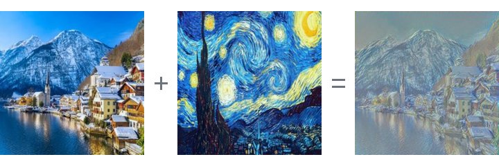
Neural style transfer
Repaint a photograph in the style of Van Gogh, Munch, Seurat or the cubists. A network trained to recognise objects separates what a picture shows from how it is painted; gradient descent then mixes the two.
Explanation and demo →
 Demo · Gaussian processes
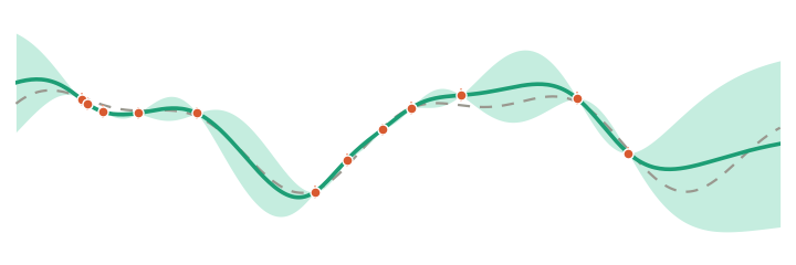
Gaussian processes
Fit a curve to a handful of noisy points and see not just the best guess but how uncertain it is between and beyond the data, and how the choice of kernel shapes both.
Explanation and demo →
 Demo · statistical mechanics
Percolation
Fill a grid at random and ask whether a connected path crosses it. The answer flips abruptly at one critical density: the simplest phase transition, simulated live with error bars from the bootstrap.
Explanation and demo →
 Demo · linear algebra
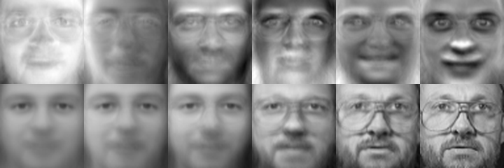
Eigenfaces
Principal component analysis finds the few directions in which faces differ most. Rebuild a photograph from a handful of these eigenfaces, see what each one changes, and mix six of them into a new face.
Explanation and demo →
 Demo · generative models
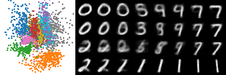
Variational autoencoders
Compress each handwritten digit to just two numbers, then drag a point around that two-dimensional map and watch the network draw the digit it decodes. Compare with a plain autoencoder to see why the variational version can generate new digits.
Explanation and demo →
6Reading
- M. Nielsen, Neural Networks and Deep Learning, free online book.
- D. J. C. MacKay, Information Theory, Inference, and Learning Algorithms (Cambridge University Press, 2003).
- C. M. Bishop, Pattern Recognition and Machine Learning (Springer, 2006).
- T. Hastie, R. Tibshirani and J. Friedman, The Elements of Statistical Learning (Springer).
- Y. S. Abu-Mostafa, M. Magdon-Ismail and H.-T. Lin, Learning from Data (AMLBook, 2012).
- K. P. Murphy, Machine Learning: A Probabilistic Perspective (MIT Press, 2012).
- P. Mehta et al., "A high-bias, low-variance introduction to machine learning for physicists", Phys. Rep. 810, 1 (2019), arXiv:1803.08823.