Simulation-Based Study of
Network Clustering and Performance Monitoring for WAN
S. Sujith Shetty
Department of Information Science and Telecommunications
School of Information Sciences
Introduction
This is a part of interim report on the NEBULA project, which focuses on an extensive simulation study of the network clustering for Wide Area Applications and the impact of performance monitoring on the network. We have simulated the whole infrastructure of the NEBULA project using OPNET Modeler 9.0 to explore various “what if” scenarios. This work was conducted by S. Sujith Shetty under supervision of Prof. Vladimir Zadorozhny.
Basic Simulation Scenario
The general scenario consists of 4 client clusters and 11 content servers scattered across North America and Europe.
The 4 client clusters are located as follows,
|
Autonomous System |
Client |
|
AS378 |
TECHNION |
|
AS27 |
UMD |
|
AS4130 |
PITT |
|
AS680 |
PASSAU |
And the 11 content servers are,
|
Autonomous System |
Server |
IP Address |
|
AS6461 |
www.apnet.com |
216.200.143.125 |
|
AS545 |
www.doi.org |
132.151.1.146 |
|
AS3561 |
www.nature.com |
216.35.73.244 |
|
AS545 |
www.handle.net |
132.151.1.145 |
|
AS17389 |
ieeexplore.ieee.org |
198.17.75.39 |
|
AS680 |
link.springer.de |
194.94.42.41 |
|
AS702 |
www.biochemj.org |
194.202.228.5 |
|
AS701 |
computer.org |
63.84.220.170 |
|
AS786 |
mirrored.ukoln.ac.uk |
138.38.146.24 |
|
AS6461 |
www.academicpress.com |
216.200.143.125 |
|
AS18713 |
www.blackwell-synergy.com |
129.41.4.140 |
Each client sends requests for a web page download every 20 minutes to all the content servers and the servers respond with the pages for download.
PATHS from each
client AS:
|
AS378 |
AS20965 |
AS3549 |
AS6461 |
|
|
|
AS378 |
AS20965 |
AS3549 |
AS701 |
AS545 |
|
|
AS378 |
AS20965 |
AS3549 |
AS3561 |
|
|
|
AS378 |
AS20965 |
AS1299 |
AS2914 |
AS13790 |
AS17389 |
|
AS378 |
AS20965 |
AS680 |
|
|
|
|
AS378 |
AS20965 |
AS1299 |
AS702 |
|
|
|
AS378 |
AS20965 |
AS3549 |
AS701 |
|
|
|
AS378 |
AS20965 |
AS786 |
|
|
|
|
AS378 |
AS20965 |
AS3549 |
AS701 |
AS18713 |
|
|
AS27 |
AS701 |
AS6461 |
|
|
|
AS27 |
AS701 |
AS3561 |
|
|
|
AS27 |
AS701 |
AS545 |
|
|
|
AS27 |
AS209 |
AS1239 |
AS13790 |
AS17389 |
|
AS27 |
AS10886 |
AS11537 |
AS20965 |
AS680 |
|
AS27 |
AS701 |
AS702 |
|
|
|
AS27 |
AS701 |
|
|
|
|
AS27 |
AS10886 |
AS11537 |
AS20965 |
AS786 |
|
AS27 |
AS701 |
AS18713 |
|
|
|
AS4130 |
AS5050 |
AS2914 |
AS6461 |
|
|
AS4130 |
AS5050 |
AS2914 |
AS3561 |
|
|
AS4130 |
AS5050 |
AS701 |
AS545 |
|
|
AS4130 |
AS5050 |
AS701 |
AS17389 |
|
|
AS4130 |
AS5050 |
AS11537 |
AS20965 |
AS680 |
|
AS4130 |
AS5050 |
AS701 |
AS702 |
|
|
AS4130 |
AS5050 |
AS701 |
|
|
|
AS4130 |
AS5050 |
AS11537 |
AS20965 |
AS786 |
|
AS4130 |
AS5050 |
AS701 |
AS18713 |
|
|
AS680 |
AS3549 |
AS701 |
AS545 |
|
|
AS680 |
AS3561 |
|
|
|
|
AS680 |
AS1299 |
AS1 |
AS13790 |
AS17389 |
|
AS680 |
AS286 |
AS702 |
|
|
|
AS680 |
AS3549 |
AS701 |
|
|
|
AS680 |
AS20965 |
AS786 |
|
|
|
AS680 |
AS6461 |
|
|
|
|
AS680 |
AS286 |
AS209 |
AS18713 |
|
Network Topology
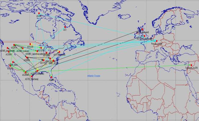
There are totally 25 subnets of which 4 contain the client clusters and 11 contain the servers and the rest are used just for routing. All routers in the network speak BGP.
The lines in black represent the paths from the Pittsburgh client cluster, the ones in yellow are for UMD, green for Technion and blue for Passau.
Node Configuration
The following settings if any have been set for optimal performance
v The routers being used are ethernet4_slip8_gtwy
v The content servers:
a) Application Supported Services
Description
§ Processing speed (bytes/sec) – 100,000,000
b) Server Setting
§ Server type - Intel SE440BX-2 (800 MHz PIII)
§ CPU - Multiprocessor (3)
§ Platform - Windows 2000
c) TCP Settings
§ Receive Buffer (bytes) - 128000
§ Window Scaling - Enabled
§ SACK - Enabled
§ Nagle Algorithm - Enabled
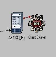
v The client clusters are 100BaseT_Lan’s
v The connections within a subnet are by 100BaseT cables
v The routers are linked by PPP_DS1 cables
TCP
Attributes
Each node with TCP as one of its contained protocols, provides an attribute, called “TCP Parameters”, to specify TCP configuration parameters. There are several preset values available for this attribute to allow you to choose from different TCP “flavors”:
Figure: TCP Parameters
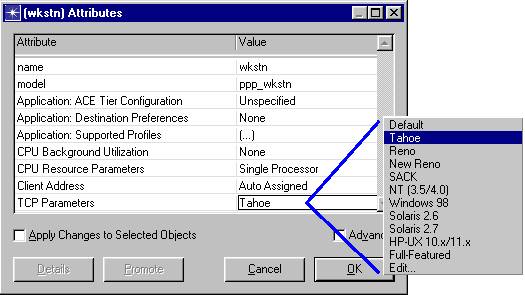
Some of the important TCP model attributes are:
- Maximum Segment Size: Defines the largest amount of data that will be transmitted as one TCP segment. Choosing a good MSS value is important because if MSS is small, network utilization may be low; on the contrary, if MSS is large, it degrades performance as it results in creation of many IP datagrams, which cannot be acknowledged or retransmitted independently. Typically, this value should be set equal to the maximum size that the “MAC” layer can handle, minus the size of TCP and IP headers. Setting this attribute to “Auto-Assigned” automatically guarantees that it is configured optimally for the data link layer over which TCP is operating.
- Receiver Buffer and Receive Buffer Usage Threshold: This is another important parameter that the application delay is sensitive to. It effects the TCP connection’s window size. Note that the window size is the amount of buffer space available in the receive buffer. This parameter determines when data should be transferred from the TCP's receive buffer to the application, thereby allowing the receive window to open further. Values are expressed as a fraction of the receive buffer size using a value between 0.0 and 1.0. In general, higher values will result in higher response times for your application (i.e., slower application).
As the receive buffer (RCV_BUFF) starts getting filled, the advertised window starts decreasing, thus limiting the flow of traffic from the peer TCP connection. A higher threshold setting will keep data in the receive buffer for a longer duration, thereby causing increased delays. Since the threshold is a fraction of the receive buffer, the effect of this setting is more observable at smaller receive buffer sizes. A low value for this setting allows data from the receive buffer to be transferred to the application more often; as a result, the advertised window is always close to the full window.
Protocol-specific Algorithms: The following algorithms are available in a given TCP implementation:
— Window Scaling
o Indicates whether this host sends the Window Scaling enabled option in its SYN message.The client host will request the Window Scaling option only if this attribute is configured as 'Enabled'. The server host will respond with the Window Scaling option enabled only if it receives the Window Scaling enabled option from the client host and this attribute on the server host is configured as either 'Enabled' or 'Passive'. Fixing the scale when the connection is opened has the advantage of lower overhead
— Selective ACKnowledgment
o Indicates whether this host sends the Selective Acknowledgement Permitted option in its SYN message. With selective acknowledgments, the data receiver can inform the sender about all segments that have arrived successfully, so the sender need retransmit only the segments that have actually been lost.
— Nagle’s Silly Window Syndrome Avoidance
o Enabling Nagle algorithm prevents small segments to be sent while the sender is waiting for data acknowledgement
— Karn’s Algorithm to avoid Retransmission Ambiguity
Terminology
Used in the Application Models
The terms commonly used in the applications model,
- Session. A session is a single conversation between a client and a server. All traffic between application clients and servers is organized into sessions. During a session, the client may alternate between periods of low traffic (lull periods) and periods of high traffic (burst periods).
- Request. A request is a packet sent from the client application to the server. A request receives a single response packet sent from the server to the client.
- Response. A response packet is sent from the server application to the client. Each request requires a certain amount of processing before the response is sent, so each application server models a single shared processor. Only one request may be processed at a time for a session, but if a server has several active sessions, each session may have a request being processed. When multiple requests are being processed, the server takes longer to respond to each request.
- Service Time. The service time for an incoming request is a function of the following factors:
— Request or response size. For certain applications (FTP get, Email receive, DB query, HTTP), the service time calculation uses response size. For all other applications, the calculation uses request size.
— Processing speed, Processing overhead, and Processing speed multiplier. These are configurable attributes for each application.
— Processor load. This is the number of active requests currently serviced by the server.
- Client-Server Addressing. The client applications have a choice of selecting either a specific node or a server node depending upon the network (i.e., local, remote, or random). For a client application to strictly communicate to a particular server, the server name attribute of the client application should be set to the TPAL address of the target server node.
- Application Details
All applications start a session at the specified application start time (100 seconds after the start of a simulation is the default). This session remains active until the specified application stop time (end of simulation is the default).
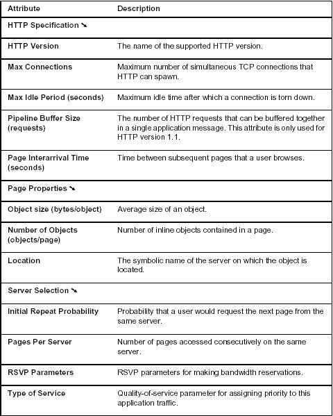
HTTP
The HTTP application models Web browsing. The user downloads a page from a remote server. The page contains text and graphic information (also referred to as “inline objects”). TCP is the default transport protocol for HTTP. Each HTTP page request may result in opening multiple TCP connections for transferring the contents of the inline objects embedded in the page. Some of the important HTTP application attributes are described below.
Configuring
Applications and Profiles
To configure a workstation or
LAN to model the behavior of a user or group of users, you need to describe
their behavior. A user's behavior or "profile" can be described by
the applications he or she uses and how long and often the applications are
used throughout the day. An application can be described in terms of its
actions, which are referred to as tasks in OPNET. OPNET provides
"global" objects for defining profiles and applications. The
advantage of using a global object is that once you have defined the profiles
and applications, you can re-use them across the entire topology. These global
objects are portable entities that are defined independent of each other and of
other objects. Therefore, you can copy and paste global objects from one
project or scenario to another and re-use the same profiles and applications.
OPNET ships with pre-defined profiles and applications that may suit the
behavior you wish to describe. You may, however, wish to modify the existing
definitions to suit your needs or even create new application and profile
definitions. This paper provides the background needed to customize and create
application and profile definitions.
Profile Configuration
Profiles describe the activity patterns of a user or group of users in terms of the applications used over a period of time. You can have several different profiles running on a given LAN or workstation. These profiles can represent different user groups - for example, you can have an Engineering profile, a Sales profile and an Administration profile to depict typical applications used for each employee group.
Profiles can execute repeatedly on the same node. OPNET enables you to configure profile repetitions to run concurrently (at the same time) or serially (one after the other).
Profiles contain a list of applications. You can configure the applications within a profile to execute in the following manner:
• at the same time
• one after the other—in a specific order you determine
• one after another—in a random order
In most cases, when describing the actions of a single user, the actions are serial since most people can only perform one activity at a time. However, when using applications that can perform non-blocking tasks, you can have more than one task running at a time. When describing the activities of a group of users, concurrency is common. Like profile repetitions, application repetitions within the profile can execute either concurrently or serially.
The Profile Definition Object defines all profiles that can be used within a scenario. Only profiles that have been defined in the Profile Definition Object can be applied to the workstations or LANs of a project and only applications that have been defined in the Application Definition Object can be used in profile definitions.
Application Configuration
A profile is constructed using different application definitions; for each application definition, you can specify usage parameters such as start time, duration and repeatability. You may have two identical applications with different usage parameters; you can use different names to identify these as two distinct application definitions. For example, the engineer may browse the web frequently in the morning but occasionally in the afternoon. Hence, you can create two different application definitions for web browsing, such as web_browsing_morning and web_browsing_noon, with two different usage patterns. You can also create application definitions based on different workgroups. For example, you may have an engineering_email and a sales_email where the former may send 3 emails/sec while the latter may send 10 emails/sec.
BGP
Border Gateway Protocol (BGP) is an interdomain routing protocol used to exchange network reachability information between BGP speaking systems. Unlike most other routing protocols that operate within an autonomous system (such as RIP and OSPF), BGP is designed to transmit routing information between different autonomous systems. The OPNET BGP model implements the current version: BGP-4.
BGP Parameters Attribute
The important attributes under BGP Parameters are described below.
Figure:
BGP Parameters Attributes Dialog Box
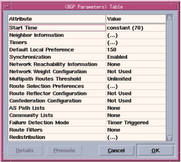
- Start Time. Specifies when the router first attempts to establish connections with its neighbors. This value should allow sufficient time for the internal gateway protocol (IGP) to have finished building its routing table. The default value of this attribute is 70 seconds. To operate correctly, this attribute must be set to the same value on all routers.
- Neighbor Information. Configures the router’s BGP neighbors. Unlike most other routing protocols, BGP does not automatically discover its neighbors. Instead, neighbors are manually configured. To configure two routers as neighbors, you can configure either one of them as the neighbor of the other. If you configure both routers as neighbors (of each other), a connection collision is detected during the simulation and one of the connections is closed, as specified in RFC 1771. The important sub-attributes used to configure Neighbor Information are described below.
Neighbor Information Box
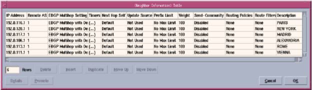
- IP Address. Specifies the neighbor’s IP address. Using the neighbor’s loopback interface address ensures that the neighboring connection remains intact as long as there is at least one route between the two routers. Otherwise, the neighboring connection closes if there is no route using the specified interface.
- Remote AS. Specifies the neighbor’s AS (Autonomous System) number. The model verifies that the specified AS number matches the neighbor’s configured AS and generates a log message if there is a discrepancy.
IP Routing Parameters
Attribute
The main IP Routing Parameters attributes affecting BGP model behavior are described below.
§
Autonomous System Number. Specifies the
autonomous system number of the router. When using confederations, this value
refers to the private AS number used within the confederation.
Configuring
BGP in a Network
This section focuses on configuring the BGP attributes described above for different types of networks. You can use the following workflow as a guide to configuring BGP. The remainder of this section contains detailed instructions for some of the major tasks presented in the workflow.
1) Assign AS numbers. A group of routers with a common set of administrative policies is called an Autonomous System (AS). Each AS is identified by a number, which you can specify on the individual routers comprising the AS. You can group the routers in your network into different ASs, each running a different interior gateway protocol (such as RIP, OSPF, or IGRP) within the AS and BGP between the border routers. AS numbers can be any integer value between 1 and 65,535. If the Autonomous System Number attribute has the default value of Auto Assigned, a random value between 1 and 65,535 is assigned to each router. For proper BGP operation, you should manually assign each BGP speaker an AS number.
2)
Configure BGP neighbors. BGP does not
automatically discover neighbors—you must specify the neighbors of each BGP
speaker. Because you specify neighbors by their IP addresses, you must first
set the address of each BGP speaker to a value other than Auto-Assigned. You
can do this by manually configuring the IP addresses or by using the
Auto-Assign IP Addresses operation. Although the model requires only that one
router of each pair of neighbors configure the other as a neighbor, configuring
both routers avoids problems by enabling the model to detect misconfigurations.
3) Configure IBGP peers. When BGP is run between routers of the same autonomous system, it is termed an Internal BGP (IBGP). If the participating routers belong to different ASs, it is an External BGP (EBGP). When a BGP speaker receives an UPDATE message from an IBGP peer, the receiving BGP speaker does not forward the routing information in the UPDATE message to other IBGP peers. Because of this, each BGP speaker needs BGP connections to all other BGP speakers in its own AS to maintain a consistent view of the routing information within the AS.
Configuring
Neighbors
To
configure two routers as neighbors, only one router needs to configure the
other as its neighbor.
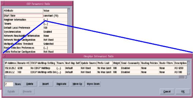
Configuring
a Neighbor of a BGP Router
- Edit the BGP Parameters . Neighbor Configuration attribute and add a row to the Neighbor Information table.
- Enter the name of the neighbor in the Description field. This value is not used in the simulation, but is available for you to enter a comment about the neighbor.
- Enter the IP address of one of the neighbor’s interfaces in the IP address field. For IBGP neighbors, use the loopback interface.
- Enter the neighbor’s remote AS. (This step is optional if the neighbor is not part of a confederation.)
- Edit the remaining attributes in the table, as necessary, except for the Routing Policies attribute
Figure: Configuring a BGP Neighbor on a Router
Experiments
Application Configuration:
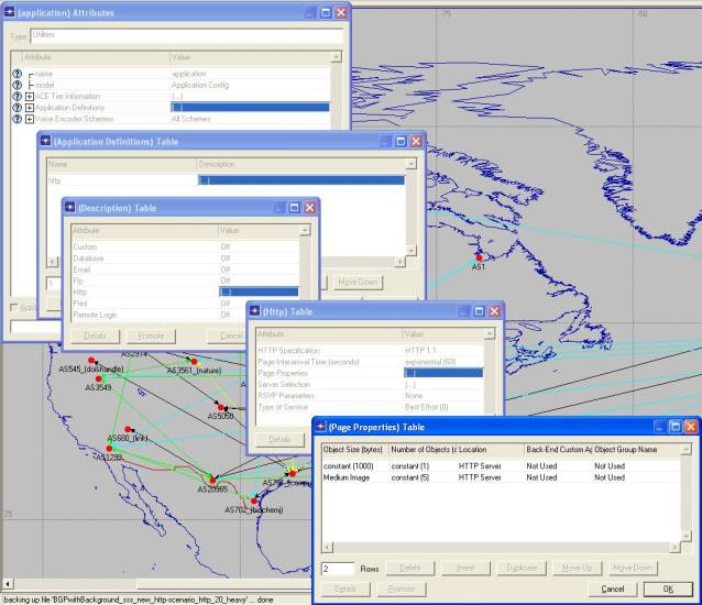
The application running on the network is a HTTP application. The application is set such that the load of the traffic is heavy. The basic function of the application is transferring web pages to the clients on request. In each server, the application name should be set in the Application Supported Services attribute.
Profile Configuration:
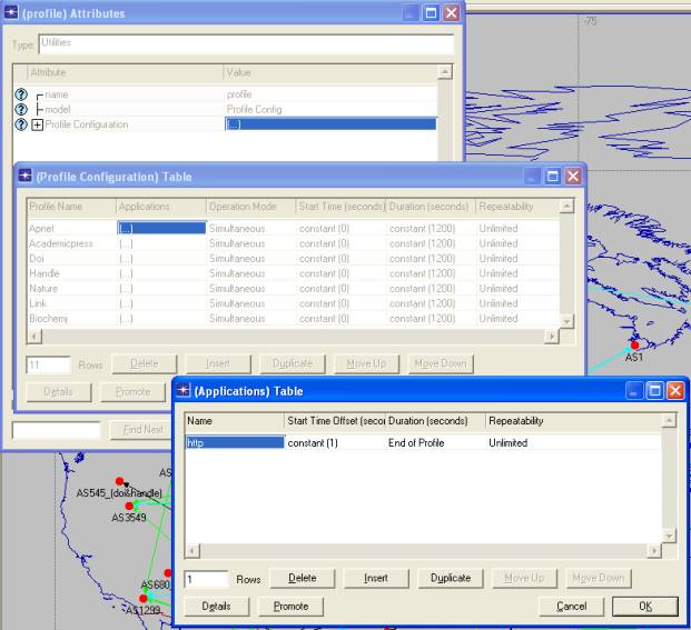
A
profile describes user behavior in terms of what applications are being used
and the amount of traffic each application generates. Profiles can be repeated
based on a "Repeatability
pattern". You can also execute more than one profile on a particular
device. A profile is created for each server. The duration of the profile is
set for 20 minutes after which it repeats until the end of the simulation. The
profile for a server is set in the Application Supported Profile attribute.
We first created three scenarios of the type mentioned as above, but with 20%, 60% and 90% background utilizations respectively. We ran each scenario for 1 hour and obtained the reports for the response times of the application for each client – server pair. We then transferred all the response time data of each scenario to separate excel worksheets. These data had to be formatted, as in invalid characters had to be removed, column names shortened and collate the data.
We then used these excel sheets of data as input to S-Plus 6.1, a statistical software analysis tool, for conducting cluster analysis. We used the Agglomerative Hierarchical Clustering method to generate the cluster plots.
Cluster analysis is the searching for groups (clusters) in the data in such a way that objects belonging to the same cluster resemble each other, whereas objects in different clusters are dissimilar.
Hierarchical algorithms proceed by combining or dividing existing groups, producing a hierarchical structure displaying the order in which groups are merged or divided. Agglomerative methods start with each observation in a separate group and proceed until all observations are in a single group.
First the excel file has to be imported into S-Plus from which a S-Plus data set is created, e.g.,
1) Import your data using File -> Import Data -> From File (e.g. Scenario20). After this is done, follow the steps mentioned below to generate the cluster plots.
2) Transpose the data using the following command by typing at the command prompt:
>Scenario20.t <- as.data.frame(t(Scenario20))
> Scenario20.t
X1 X2 X3 X4
X5
Technion.Apnet 214.85932 260.48534 304.030017 293.093721
34.562773
Technion.Blackwell 72.73693 235.16951 283.127462 316.299320
35.445702
Technion.Academicpress 16.79730 166.63817 262.832641 309.427988
324.752655
Technion.Doi 59.16718 117.30579 162.424421 233.326323
272.766040
.....
Now use the new transposed data 'Scenario20.t' to cluster
3) Cluster the data using the function agnes(). Type at the command prompt:
> my.agnes <- agnes(Scenario20.t)
> summary(my.agnes)
> plot(my.agnes)
The resultant cluster plots are generated for each of the scenarios. The x-axis legend is seconds and the y-axis legend is the client – server pair.
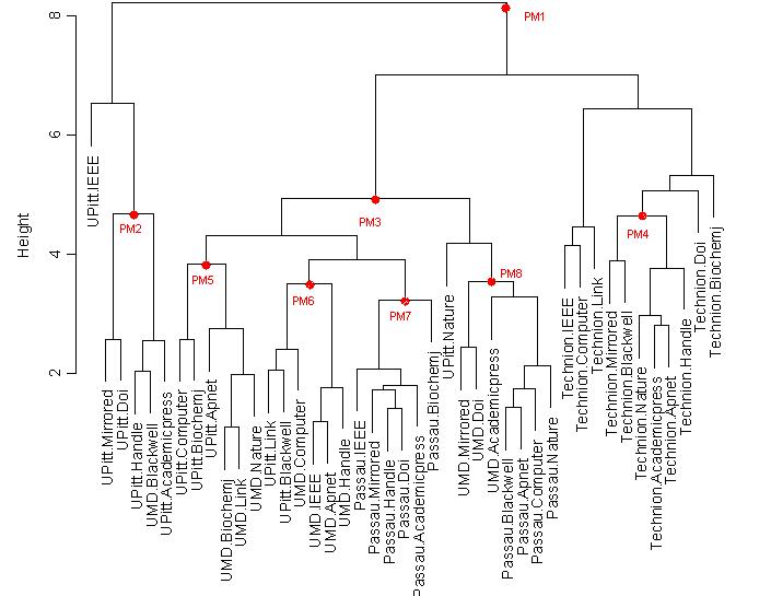
HTTP (Heavy) with 20% Background Traffic
This cluster plot shows that there are four main clusters. The first one is dominated by the client UPitt. The second cluster is dominated by UMD, the third by Passau and the fourth by Technion. Whats very evident is that, only in the Technion cluster all the client-server pairs are close to each other. In all the other clusters, some client-server pairs are distant. For example, UPitt is found in clusters one, two, three and five with concentration in cluster one. Similarly, UMD is found in clusters one, two, three and five with concentration in cluster three. Passau is found in clusters four and five and dominates cluster four completely. Technion completely dominates cluster five.
HTTP (Heavy) with 60% Background Traffic
In this cluster plot we see that only Technion-server pairs are closely packed and form a cluster. Passau-server pairs also form a close cluster except for one stray case which is Passau-Handle. All the other client-server pairs are spread out and there’s not much of dominance of any particular client or server in the other clusters.
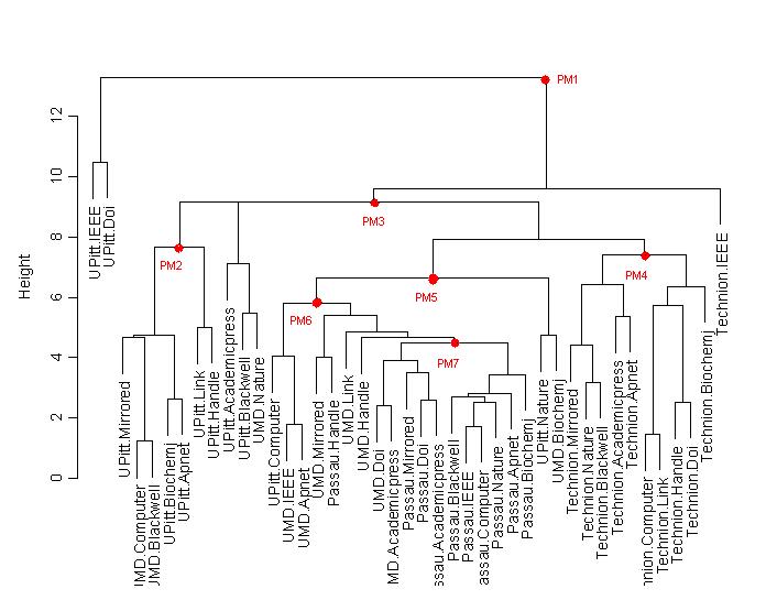
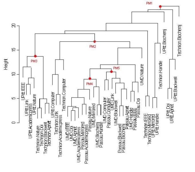
HTTP with 90% Background Utilization
In this plot, it is clear that there are many small pockets of clusters of single client and multiple servers. The client-server pairs of none of the clients are all together. This can be attributed to the high 90% background utilization.
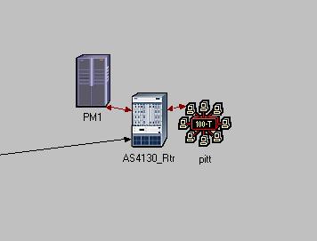
Analyzing the cluster plots carefully, I’ve placed performance monitors at various clusters. The performance monitors (PM’s) are basically servers of the same configuration as the content servers. These PM’s act as a repository of the latency profiles. Now each client sends a request for download of light HTML page to the PM in its cluster before sending a request to the content servers, but these requests to the PM’s are at a much lower frequency, say 3 requests every 20 minutes. Each PM, in turn sends a request to the higher level PM’s that it is connected to in the cluster plot.
So now, we created 3 more scenarios like the first 3 three with the added performance monitors for the clusters.
These simulations encapsulate the concept of placing PM’s with the latency profiles in a network load analysis point of view.
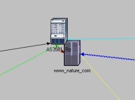
Snapshot of a PM in a client AS:
The cluster plots with PM’s:
HTTP with 20% Background Utilization with
PM’s
HTTP with 60% Background Utilization with PM’s
HTTP with 90% Background Utilization with
PM’s
Placement of PM’s :
We placed the PM’s based on the following criteria:
1. The client-server clusters formed
2. Size of the clusters. If too small then have a common PM for more than one cluster
3. Place the PM in the dominant client or dominant server
4. If more than one client or server locations that are suitable for placement are there, then just choose any one.
5.
We created separate applications and profiles for each of the PM’s. The PM’s are connected to the routers in the respective AS’s using 100BaseT cables.
The following comparison graphs give a clear picture,
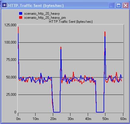
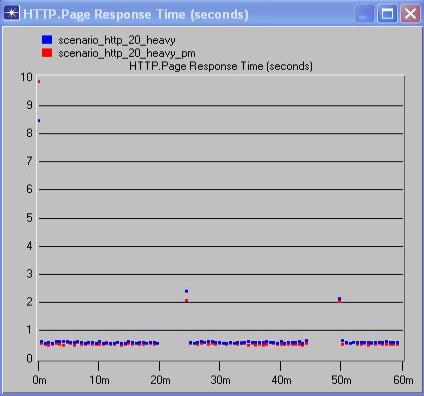
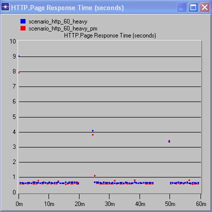
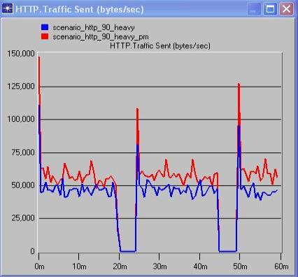
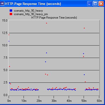
From the above comparison graphs of traffic and response times, between scenarios with and without PM’s but with same background traffic, it is possible to analyze the effect of PM’s on the network.
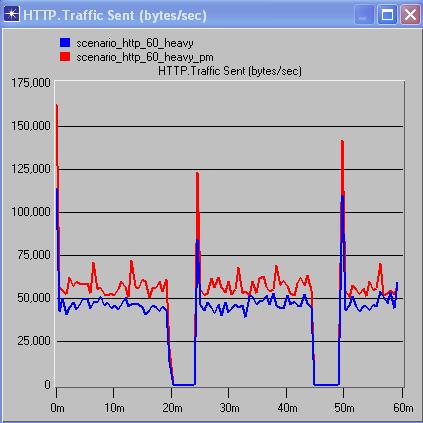
The above comparison graphs show that for the scenarios with 20% background utilization, there’s not much of a noticeable difference in the traffic and correspondingly barely noticeable difference in the response times of the application. In the 60% background utilization graphs, we see that although there’s an increase in the traffic load, the variance in the response times is barely noticeable.
The 90% background utilization graphs show an increase in load with the addition of PM’s but still have a relatively low variance in response times. The vast difference between the 20% scenarios and the 60% and 90% scenarios in the traffic sent is something that puzzles me. WE can’t place a finger as to why this happens. This could be attributed to the way OPNET functions. We conclude my analysis stating that the addition of PM’s seems feasible as the tradeoff between traffic load and response times is negligible, in other words, the additional load of the PM’s have not significantly increased the response times.
Future
Research:
Simulating the process of acquiring the latency profiles and then conducting an overall more precise analysis of the impact of PM’s on WAA’s.
We were initially importing traffic into my model using external traffic files, which were in the format shown below and wrote a script in Java to parse the data. But the import of traffic was not feasible, so that way of representing traffic was scrapped.
References:
1). L. Raschid, H.F. Wang, A. Gal, V. Zadorozhny. Latency Profiles: Performance Monitoring for Wide Area Applications
2). OPNET Product Documentation
3). http://www.psc.edu/networking/perf_tune.html
4).
H. Charles Romesburg: Cluster Analysis for Researchers
5).
S-Plus system documentation