| HPS 0628 | Paradox | |
Back to doc list
Paradoxes of Impossibility: Computation
John D. Norton
Department of History and Philosophy of Science
University of Pittsburgh
http://www.pitt.edu/~jdnorton
We live in the age of computers. As one aspect after another of our lives is turned over to computers, it seems as if there is nothing that lies beyond their powers.
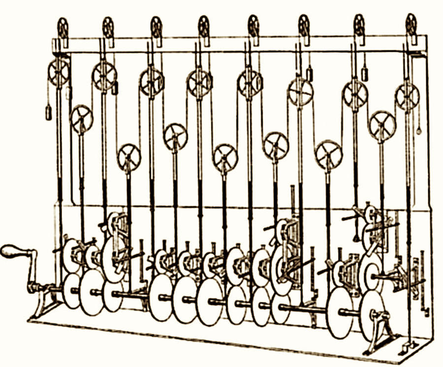
In 1882, William Thomson designed a computing
machine for predicting tides.
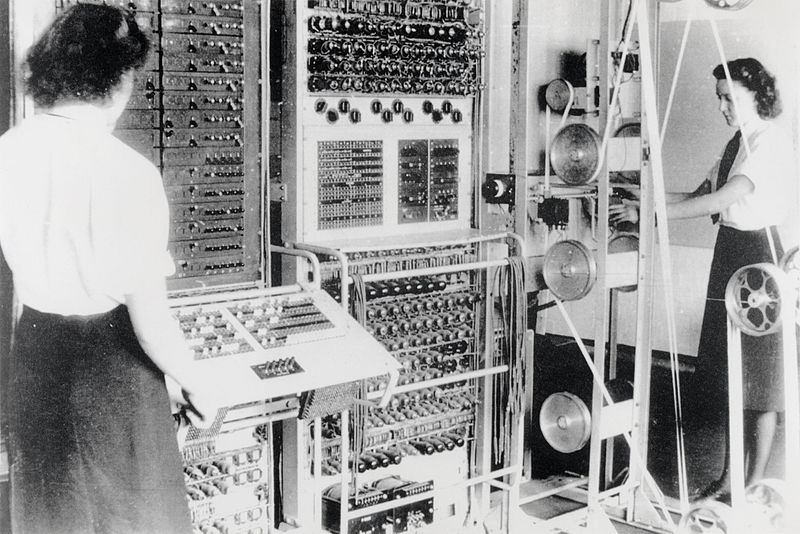
In World War II, the Colossus computing machine was
devised by mathematicians at Bletchley Park for breaking German Enigma
codes. Here is a Colossus Mark 2 computer, operated by Dorothy Du Boisson
(left) and Elsie Booker (right), 1943.
https://commons.wikimedia.org/wiki/File:Colossus.jpg
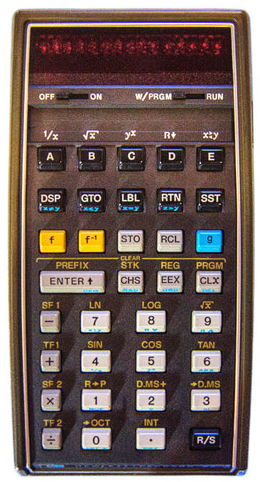
The HP-65 was the first hand-held programmable
calculator. In 1975, it was taken on the Apollo=Soyuz test mission and was
the first such device in space. It was taken as a backup to the onboard
computer, but was not needed. Its program memory could hold 100
instructions, each of 6 bits in size. The programs were stored on small,
magnetically coated cards. Today's cell phones have vastly more computing
power.
https://commons.wikimedia.org/wiki/File:HP-65.jpg
It seems that our computing horizons are unlimited. All we need are machines with more storage and faster processors and there is nothing beyond their computational powers. What we shall see in this chapter, however, that this is not so. Even given the most liberal of capacities in both time and space, there are many problems that no computer can solve, as a matter of principle. Indeed, in a sense that we can make precise, most problems cannot be solved by them.
It is not a matter of trying a little harder, or of handing the problem over to the next generation of machines that that run so much faster than the last generation's. None of this will help. There are problems that are as insoluble to computers as the squaring of the circle is to straight edge and compass constructions. The analysis will employ notions developed in earlier chapters. Most important among them will be the analysis of different sizes of infinities and the use of self-referential diagonalization arguments.


Proving the impossibility of the classic geometric constructions of the last chapter was a major achievement of nineteenth century mathematics. Their solutions became part of the origin of group theory. This powerful theory figures prominently today in advanced physics and elsewhere.
Questions such as will be investigated in this chapter played a corresponding role in the development of twentieth century mathematics. That certain well-defined computational tasks go beyond what any computer can achieve is one of a large collection of results that limit the reach of formal methods.
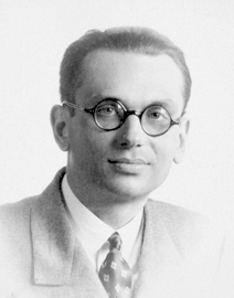
https://en.wikipedia.org/wiki/File:Kurt_gödel.jpg
The best known of these is Kurt Goedel's demonstration of the incompleteness of arithmetic. He showed that any consistent axiom system for ordinary arithmetic necessarily fails to capture all the truths of arithmetic. There will always be truths of arithmetic that the system can neither prove are true or prove false. The import of the result goes far beyond arithmetic. We learn from it that any formal system powerful enough to host arithmetic is incomplete. The long-appealing idea, extending as far back as Euclid's Elements, was that branches of science could have all their content captured by carefully chosen, finite list of axioms. Goedel showed this idea fails.
Goedel's celebrated analysis depends essential on a sophisticated use of self-reference. We shall see here that self-reference again has a central role in the demonstration of the existence of uncomputable tasks.
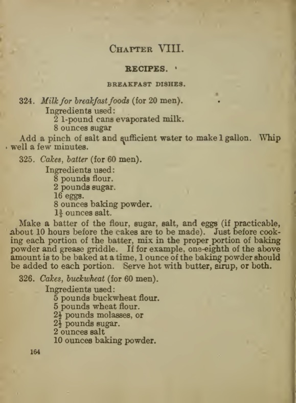
Our goal is to deduce principled limitations on what computation can achieve. To arrive at precise results, we need a precise characterization of what we ask computers to do. The first step in forming this precise characterization is to introduce the notion of an effective method. They are what is implemented as algorithms in the simplest and one of the most important categories of computation. The informal idea for such a method is that it is a set of instructions that can be followed to the desired end without needing any special human insight. Just follow the steps specified and a good result is assured.
The simplest version of this in ordinary life is a really good recipe for cooking. It must be so complete as to leave no room for imagination or invention.
Here is a different sort of instruction set.

https://commons.wikimedia.org/wiki/File:Canada_Right_Shoulder_Pedestrian_Signal_Instruction_Sign.svg
These are conditions that an effective method must meet:
An effective method or algorithm is a finite
set of instructions such that:
1. If the instructions are followed
correctly, they must give the right answer (and no wrong answers).
2. They give the right answer after
finitely many steps.
3. Their implementation is purely
mechanical and requires no insight or imagination.
To illustrate these conditions, here are a few cases of failure; and a success.
The
day after Sunday is:
(check all that apply)
(a) Monday
(b)
Tuesday
(c)
Wednesday
(d)
Thursday
(e)
Onions
In response to a multiple
choice examination, with possible answers (a), (b), (c), (d) and
(e):
Answer to question 1: (a) whatever the question.
Answer to question 2: (a) whatever the question.
Answer to question 3: (a) whatever the question.
etc.
FAILURE: Condition 1. requires that the method never give wrong
answers. This one will give mostly wrong answers.
Sinking ship image:
https://commons.wikimedia.org/wiki/File:Sinking_of_the_Lusitania_London_Illus_News.jpg
fireworks:
https://commons.wikimedia.org/wiki/File:Bratislava_New_Year_Fireworks.jpg
x
= 2x
To find a number greater than zero equal
to twice itself:
Compare 1 with 2x1.
Then compare 2 with 2x2.
Then compare 3 with 2x3.
Then compare 4 with 2x4.
etc.
FAILURE: Since there is no number greater than zero
with this property, this method leads to the computer to continue
indefinitely without ever halting and reporting failure. Condition 2.
requires the method to halt after finitely many steps.
6
= 1 + 2 + 3
To find a perfect number:
Pick a number and check if it is equal to the sum of its factors,
excluding itself.
If it is, halt; if not, repeat.
FAILURE: Condition 3 requires mechanical
implementation, without the need for insight or imagination. The recipe
fails to say how the number for test is to be chosen. (Condition
1 is also violated since there is no assurance that the procedure will
halt in finitely many steps.)
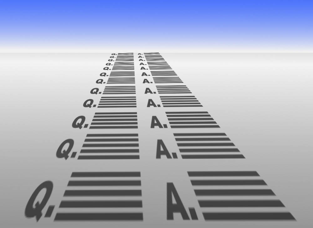
An infinite look-up table.
Here is a method of having a computer speak a language. We make a table
that has every possible question that could be asked in the first column;
and the appropriate answer in the second. Since questions and answers can
have arbitrary length, the table must be infinite in size. To answer a
question, the computer finds the question asked in the table and then
returns the corresponding answer.
FAILURE: An effective method employs finitely
many instructions. This infinite look up table is equivalent to
an infinity of individual instructions.
60
= 2 x
2 x
3 x
5
Find all the factors
of a given natural number n:
Test for divisibility by 1.
Test for divisibility by 2.
Test for divisibility by 3.
...
Test for divisibility by n.
Report all divisors

SUCCESS: The procedure halts after finitely many steps (n); it
gives a answer and only a correct answer; and it requires no insight or
imagination.
This notion of effective method will be examined more closely below. It does not exhaust the methods used profitably in real applications in computer science. For example, a solution may be sought in a very complicated space of possible solutions, such as one with very high dimensions. An effective method that assuredly finds the best answer may be computationally prohibitive. However a random walk in the space may produce a result that is good enough for real-world purposes. In a random walk, we explore the solution space, taking steps chosen by some probabilistic randomizer.
Consider again Condition 2 above for an effective method.
2. They [the instructions] give the right answer after finitely many steps.
It contains an important fact about the theory of computation. We have seen in earlier chapters that there is no incoherence in the idea of the completion of infinitely many actions. This completion, however, is not something within the reach of our ordinary physical methods. That means that it is a physical condition as opposed to a logical or mathematically founded restriction. We can conceive physical systems in which it is possible for an infinity of actions, or an infinity of computational steps to be completed in a finite time. In such systems, tasks that are deemed uncomputable in the theory of this chapter may become computable.

The simplest scheme just involves a computer than
can accelerate its operation of each step without limit. A more exotic
example of such a system is found in what have been called "Malament-Hogarth
spacetimes." Such a spacetime is shown in the figure above. It is a
spacetime with unusual properties. The worldline of
the calculator C is of infinite proper time. Loosely speaking,
the calculator experiences an infinity of time along the curve shown, even
though it has an upper bound in the figure. The calculator C could then
carry out an infinity of calculations, such as checking that every even
number 2, 4, 6, ... has some property. The calculator could then signal
the result of each test to the observer O. In this spacetime, only finite
proper time elapses along the segment of the world line of O in which the
signals are received.
The notion of an effective method is a first step towards a more precise, general notion of a computation and a computer. While the idea is informally easy to grasp, there are many ambiguities in it. Exactly what counts as an instruction? What is to be "mechanical"? Is there a machine with definite states that implements the instructions? What sorts of states does the machine have and how does it move from state to state?
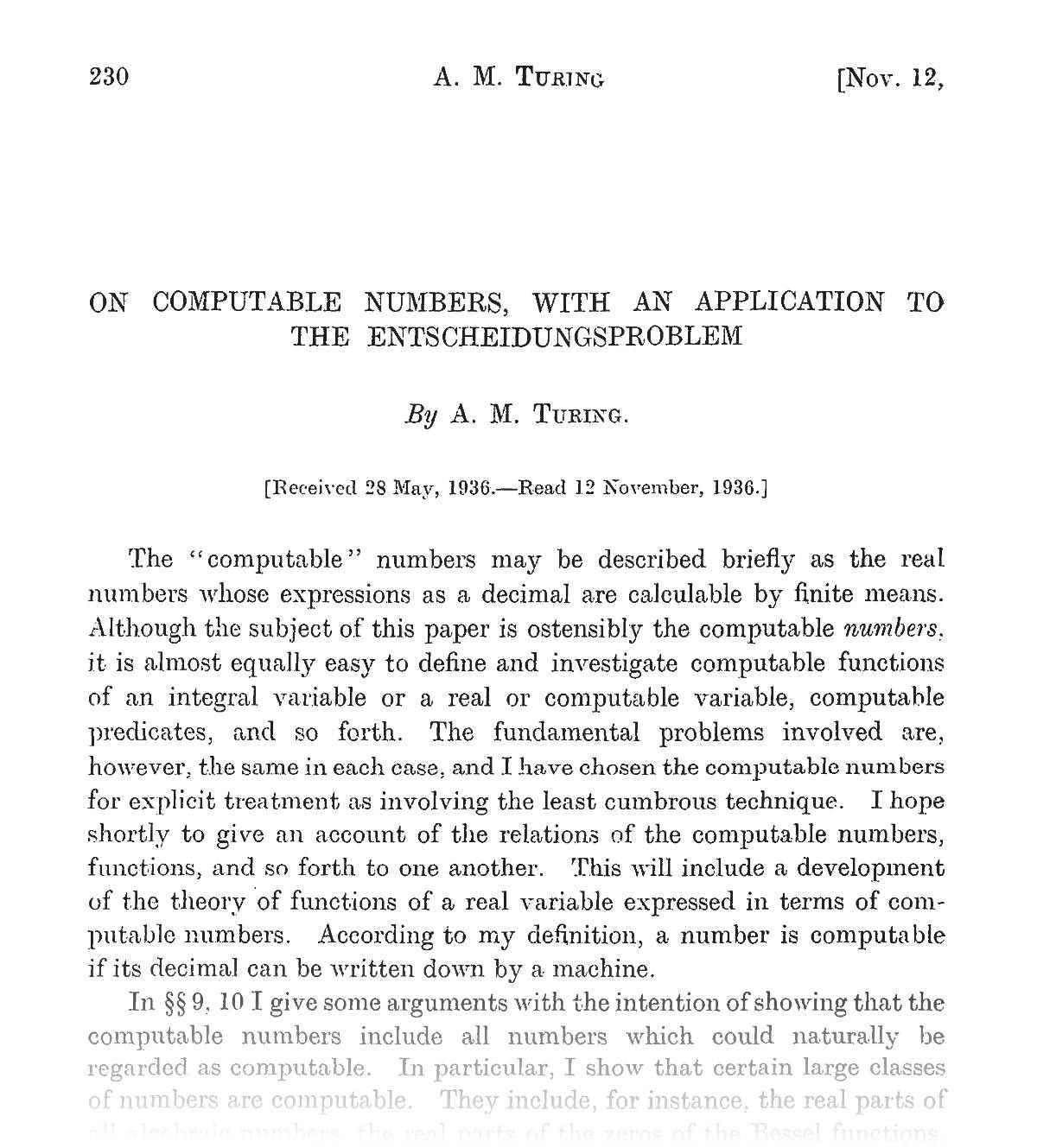
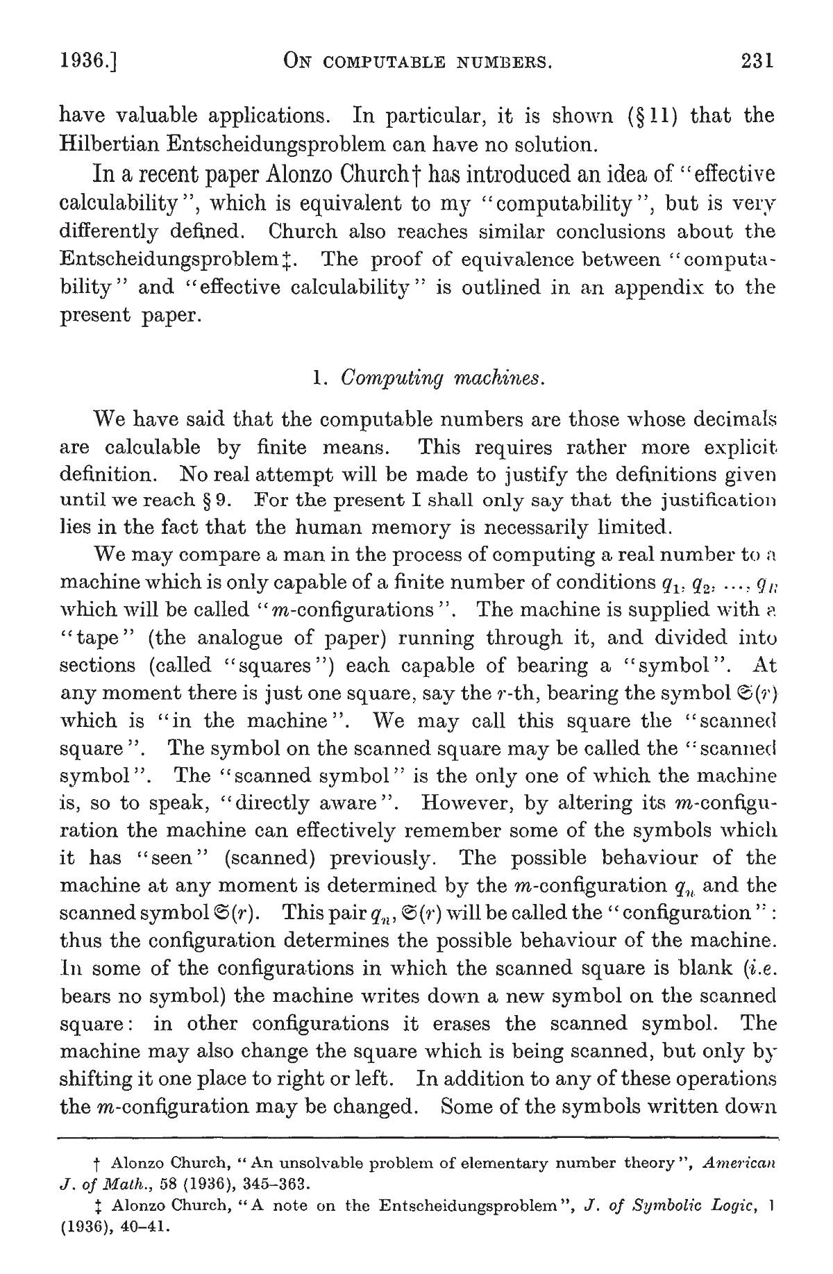
In order to escape these ambiguities, theorists in the early to mid twentieth century produced several more precise specifications. The best known and easiest to grasp is the idealized machine introduced by Alan Turing in his 1936 paper "On Computable Numbers with an application to the Entscheidungsproblem [decision problem]."
There are two basic elements of the machine. First is a paper tape that is of unlimited length and is divided into cells. Second is a head, the computing part of the machine, that moves left and right along the tape. The tape needs to be of unlimited length so that the head never runs out of tape as it moves along the tape.

We would now imagine that head to be stationary and the tape to be fed through it. However, in 1936, Turing was still imagining as a model for his machine how a person might use paper for calculations. The paper is fixed in place and person moves along it, pencil in hand, writing symbols. The term "computer" was then undergoing a transition from meaning "person who computes" to "machine that computes."
The tape cells can carry symbols, drawn from some finite alphabet, such as A, B, C, ..., Z; and cells can also be blank.

The computing head can adopt any of a finite number of states, 1, 2, 3, ..., N.

As the head moves along the tape, it can
do the following:
Read the content of current cell.
Write a symbol in the current cell, possibly overwriting
the current cell's content; or erase the content of the current cell,
leaving it blank.
Move one cell to the left (L) or the right (R).

Which it does is determined by a program. The program consists of a finite set of lines of code. Each line has five symbols with the following meanings:
|
Current state of the head |
If this symbol is read in the current cell... |
...then write this symbol into the cell. |
Move L or R |
Adopt this new state |
For example
1 A
B R 2
means "If you are in state 1 and read symbol A in the current cell, write symbol B in the current cell and move one cell right R. Then adopt state 2."
The key fact is a that a program consists of a
finite list of instructions of this type.
A Turing machine computes by transforming the state of the tape. We provide an input to the machine by specifying the initial tape configuration. We then set the programmed head on the tape in some appropriate initial cell and allow it to run.
The condition for halting
is that the head arrives at a state such that there is no instruction for
the current cell or no state in the program. For example, the head may be
instructed to move to state 10, when state 10 does not figure in any
instructions in the program. Or, if the head is in state 1 and has arrived
at a cell with symbol C, it expects to find an instruction that looks like
1
C something something something
If there is no such instruction in the program, the head halts and this
final state of the tape is the output of the program.
Here are some simple programs for the machine.
The input tape is blank everywhere except for a finite sequence of cells, each with the symbol A.
(initial) ... blank blank A A A A A blank blank ...
The program has two lines:
1 A blank R 1
1 blank blank R 2
The head is set initially on the leftmost A in state 1. When in state 1, the head erases an A in the current cell and moves to the right, remaining in state 1. It repeats this action as long as there is an A in the current cell. When all the A's have been erased, it moves to state 2. Since there is no line of code for state 2, the head halts. The output tape is blank.
(final) ... blank blank blank blank blank ...
To add 4 + 3, the initial state of the tape is everywhere blank except for 4 A's in a row, a blank and then 3 A's.
(initial) ... blank blank A A A A blank A A A blank blank...
The program is
1 A blank R 2
2 A A R 2
2 blank A R 3
The head is initial placed on the leftmost A in state 1. The first step of the program is to erase the leftmost A:
(intermediate) ... blank blank blank A A A blank A A A blank blank...
It then moves to state 2. As long as the head reads an A in current cell, it leaves the A there and moves one cell to the right. Eventually it finds the blank cell between the two sequences of A's. It replaces that blank with an A, moves right and adopts state 3. Since there are no lines of code for state 3, the execution halts with the tape:
(final) ... blank blank blank A A A A A A A blank blank...
Overall, effect is an addition: the initial tape had 3 + 4 A's and the final tape had 7 A's.
Here is a simple program that fails to halt. The tape is everywhere blank and will remain blank in the course of the computation.
... blank blank blank blank blank...
The program has two lines:
1 blank blank R 2
2 blank blank L 1
The head can start in state 1 on any cell. The overall effect is that the head oscillates R, L, R, L, R, ..., never halting. If a program like this were to be executed on a real computer, we would say the computer has "crashed" or "frozen."
The lowest level capacities of a Turing machine are very meager and the computational tasks programmed above are rudimentary. It is not intended to be a design for practical use. In practice, its use would be cumbersome and inefficient. Rather, the extreme simplicity of the design makes it amenable to general theoretical analysis. Results about the capacities of a Turing machine are easy to obtain precisely because the machine is so simple.
However a Turing machine is quite capable of carrying out rich and complicated computational tasks. The key fact is that the tape can be extended indefinitely, so there is no limit to its storage capacity; and the only time restriction is that the computation must be completed in finitely many steps. These finitely many steps, however, can be very, very large. While the programs that allow a Turing machine to do something interesting may be huge and unwieldy, all that matters is that the machine can be programmed to carry them out.
How does the computational reach of a Turing machine compare with other sorts of digitally based computation systems?
Many different schemes have been devised to model idealized computers. We might even imagine one for ourselves. Take the computer you normally use. What if it were supplied with an unlimited amount of memory and you placed no limit on how long you are prepared to wait for an answer? Its capacities provide another way to prescribe what is computable.

We might suspect that each plausible implementation of an idealized computer would lead to a different sense of what is computable. We might wonder if one implementation is good at, say, arithmetic. Another might be good at language processing; and another at image processing. That would lead to different senses of what is computable:
Computable sense 1 on idealized computer of type 1.
Computable sense 2 on idealized computer of type 2.
Computable sense 3 on idealized computer of type 3.
...
What Alan Turing, the logician Alonzo Church and others realized, however, was that all the different schemes they devised of idealized computers had exactly the same computational reach. That is:
Church-Turing thesis: All computers that realize effective methods can compute the same things.
 =
=  =
= 
If some computer system is identified as having the "power of a Turing machine," we are informed that it implements effective methods and performs at the level of all these machines.
Evidence for the thesis came through elaborate demonstrations that one scheme after another could be shown to have the same capacities.
Ultimately, however, the thesis is not something that can be proved, like a theorem in arithmetic. For the characterization of an effective methods is imprecise. However, in the years since Church and Turing worked, more positive instances have come to light and no counter examples have been found.
The result is, perhaps, not so surprising if we reflect on how fancy, modern digital computers operate. At their lowest level, they have a huge number of memory storage devices that can hold a bit, a "O" or a "1"; and circuitry that can shuffle the bits around. And that is all. At that level, they do not seem so different from a Turing machine.
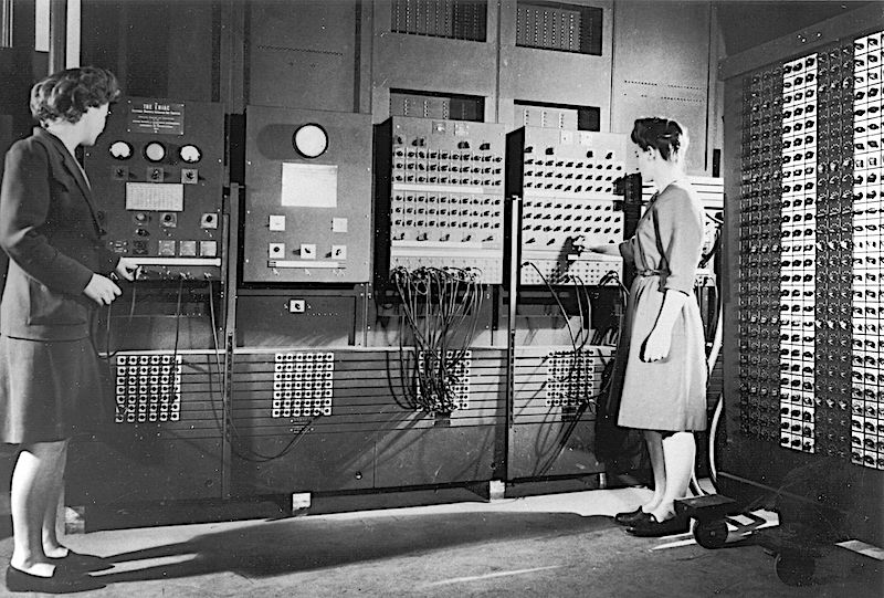
ENIAC, one of the
first digital computers from the mid 1940s.
https://commons.wikimedia.org/wiki/File:Two_women_operating_ENIAC.gif
Here is the description of
this photo from the wikimedia
commons source:
" Two women operating the ENIAC's
main control panel while the machine was still located at the Moore
School. "U.S. Army Photo" from the archives of the ARL Technical Library.
Left: Betty Jennings (Mrs. Bartik) Right: Frances Bilas (Mrs. Spence)
setting up the ENIAC. Betty has her left hand moving some dials on a panel
while Frances is turning a dial on the master programmer. There is a
portable function table C resting on a cart with wheels on the right side
of the image. Text on piece of paper affixed to verso side reads "Picture
27 Miss Betty Jennings and Miss Frances Bilas (right) setting up a part of
the ENIAC. Miss Bilas is arranging the program settings on the Master
Programmer. Note the portable function table on her right.". Written in
pencil on small white round label on original protective sleeve was
"1108-6". "
The Church-Turing proceeds with a reasonable, but unrealistic assumption. It is that all the computing devices considered operate with the same freedom as the highly idealized Turing machine. That is, it is assumed that they have unlimited memories and there is no limit on the time that can be taken to compute its result, as long as that time is finite.
This means that real computers--the sort we work with day to day--are less powerful than a Turing machine. None of our machines can function for an unlimited time. Their components will eventually wear out and fail. Long before then, we likely have lost patience waiting for the result. The restriction from the limit to a finite memory is easiest to see. Consider some enormous addition problem: add two absolutely huge numbers together:
12345... + 5678...= ???
No matter how much memory some particular real computer has, there will be some addition problem that it cannot solve. It simply will not have enough memory to store all the digits of the very, very, very large addition problem. By assumption, a Turing machine has no such limit. Its tape can be extended as much as is needed for any such addition problem.
We need one final step to represent the behavior of computing machines.
The input to a Turing machine is a finite sequence of symbols on the machine's tape. The sequence may be of arbitrarily great length, but it will always be finite. There will be an infinity of them. The possible inputs will include tapes with:
A or AA
or AAA or AAAA
or AAAAA or ...
In principle, we could have much fancier input tapes such as:
WHAT IS THE SQUARE ROOT OF SIXTY-FOUR?
Since the possible symbols are drawn from a finite set, it follows that the number of possible inputs is countable. that means that we can assign a unique natural number to each possible tape input.
It is not immediately
obvious that this numbering is possible. There are many schemes that
implement it. A simple one is Goedel numbering.
We first number the symbols: blank=1, A=2, B=3, ... We then take the input
string and convert it to a sequence of numbers:
blank blank B A A ...
becomes
1 - 1 - 3 - 2 - 2 - ...
This sequence of numbers is then matched to the sequence of prime numbers
2 - 3 - 5 - 7 - 11 - ...
and we form a huge composite number
21 x 31 x 53 x 72 x 112
x ...
This number then uniquely encodes the original input string. The
uniqueness is guaranteed by the fundamental theorem of arithmetic. It
tells us that each composite number has a unique factorization into a
produce of prime numbers.
The output of a Turing machine is also a finite sequence of symbols on the tape. Correspondingly, this output may also be encoded by a unique natural number.
Finally, the operation of the Turning machine is to map the input to the output, that is, the operation can be represented as function that maps a natural number (the code of the input) to a natural number (the code of the output). This set of functions is the set of "computable functions."
Here's how the operation looks:
Input with code number 314159.
| Input acted on by computable function f |
↓ | |

Input with code number 314159 leads to output 2718 = f(314159).
Similarly, each computer program consists of a finite list of instructions. For example, the adding program above for a Turing machine consists of the program:
1 A blank R 2
2 A A R 2
2 blank A R 3
Since each instruction consists of 5 symbols, we can turn this program into one long list:
1 A blank R 2 2 A A R 2 2 blank A R 3
By using the encoding techniques above, this list can be given a unique natural number. It follows that each computer program can be assigned its own unique natural number. The set of programs, then, is countably infinite.
It is not a great stretch to see how this characterization applies to a Turing machine. However, in the light of the Church-Turing thesis, this same characterization applies to all digital computer systems that implement effective methods.
By similar considerations, all the operations of a digital computer can be reduced to functions on the natural numbers.
Consider, for example, a computer system that takes as input all the data pertinent to a rocket to be launched to Mars. The task is to find the appropriate trajectory. All its input comprises a finite amount of digital data that can encoded a single number. The output of the program is also a finite amount of digital data that can be encoded by a single number. Hence the operation of the computer is reducible to a function that maps the number encoding the input to the number encoding the output.
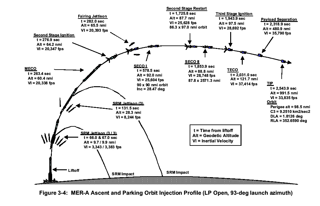
The figure shows key events during the 2003 launch by NASA of the Mars Exploration Rovers. Image: https://mars.nasa.gov/mer/mission/timeline/launch/launch-diagram/
A computer may translate all of Shakespeare's plays into another language. The entirety of the plays is just a long sequence of symbols that can be encoded by a single number; and the same is true of the translated version.
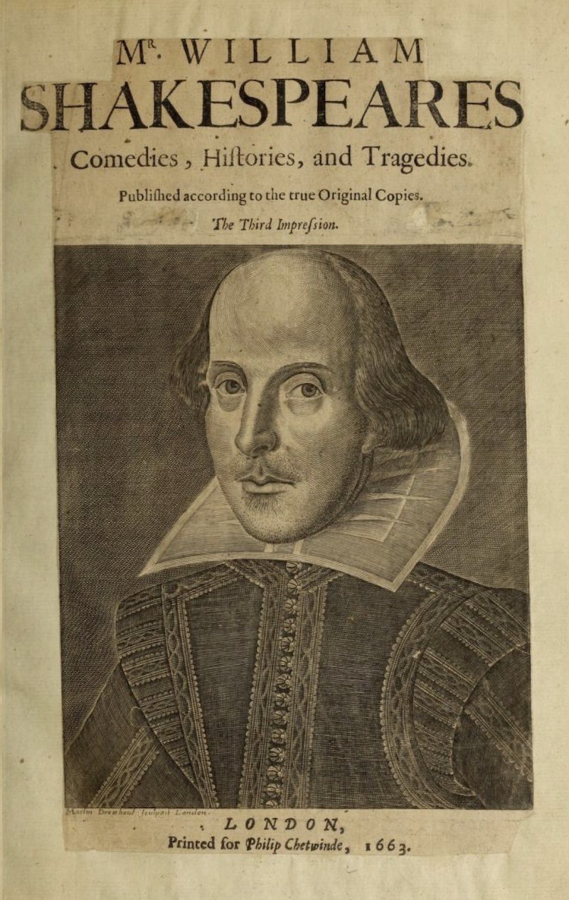
Image manipulation software takes as input an image encoded in a computer file as a long sequence of digital data. Each pixel is just a few numbers in a file that encodes the brightness and color of the pixel. If its output is another image, that image is also just a long sequence of digital data. Once again, the operation of the software can be represented by a function on the numbers encoding each sequence.
![]()
In sum:
An effective method can be represented by a computable function that maps natural numbers to natural numbers.
How many computation functions are there? Every program for any digital computer consists of computer files written in some symbolic language. Every program consists of a finite list of instructions, where each instruction consisting of some finite list of symbols. That is, if we string all the instructions together, each program consists of a finite string of symbols, possibly very long. This is general. Whatever the computer language, every program is, ultimately, a finite sequence of symbols.
Using the same methods as used on the inputs and outputs, we can encode each program by a unique natural number. We conclude:
There is a countable infinity of computable functions.
We can now ask the most fundamental question:
Are there tasks no computer can perform?
We have converted that into the more precise question:
Are there tasks that cannot be completed by an effective method?
This question in turn becomes the still more precise question:
Are there tasks that cannot be completed by a Turing machine?
And then finally, the question becomes:
Are there functions from natural numbers to natural numbers that are not computable?
The answer is easily given: there are such functions that are not computable. This is shown by a diagonalization argument. We will assume, for the purpose of a reductio argument, that there is computer program that computes each function from natural numbers to natural numbers. Since computer programs form a countably infinite set, it follows that the set of functions is countable and can be enumerated. Each computer program is encoded by a natural number, 1, 2, 3, .... and each computer task is implemented by a function we can label with natural numbers, 1, 2, 3, ..., according to the computer program that computes it:
That is we have:
function number ↔ specific
program
function ↔ task undertaken
We put these numbers and functions in a table.
• Each row encodes a particular function. Each function maps 1 to some value, 2 to some value, 3 to some value, and so on. These values f(1), f(2), f(3), ... form a row
• Each row is labeled by the code number of the program that executes the function in the row.
We end up with a table that looks something like this:
| Function number | f(1) | f(2) | f(3) | f(4) | f(5) |
f(6) |
f(7) |
f(8) |
... |
| 1 |
3 |
32 |
28 |
5 |
781 |
34 |
480 |
93 |
... |
| 2 |
14 |
38 |
841 |
820 |
640 |
825 |
86 |
844 |
... |
| 3 |
159 |
462 |
9 |
97 |
62 |
3 |
5 |
60 |
... |
| 4 |
26 |
6 |
71 |
4 |
8 |
421 |
132 |
95 |
... |
| 5 |
5 |
43 |
69 |
944 |
620 |
170 |
82 |
505 |
... |
| 6 |
358 |
832 |
399 |
5 |
89 |
67 |
306 |
82 |
... |
| 7 |
97 |
7 |
375 |
92 |
98 |
9 |
64 |
231 |
... |
| 8 |
9 |
950 |
10 |
30 |
628 |
821 |
70 |
72 |
... |
| ... |
... |
... |
... |
... |
... |
... |
... |
... |
... |
We can now construct a function that differs from any function in the table merely by adding one to the shaded numbers along the diagonal. That is, we form
f(1) = 4
f(2) = 39
f(3) = 10
...
f(8) = 73
...
This new function cannot appear anywhere in the table since it differs by construction on one value with each of the functions in the table. It is an uncomputable function. That is, it represents a computational task that cannot be carried out by any computer whose operation is encoded in functions on natural numbers as in the table. For any encoding system we specify, this diagonalization construction will produce a task that the computer cannot carry out.
This construction yields one uncomputable task. How many more of them are there? The answer is infinitely many more:
The set of computable functions is countable.
The set of functions is uncountable.
"Function" here is restricted to functions from natural numbers to natural numbers.
This immediately translates into cardinality conditions on the operation of computers:
The set of computer programs is countable.
The set of computational tasks is uncountable.
There are, it follows, vastly more tasks we might ask a computer to perform than there are programs that can perform them.
To see this, we need only show that the set of all functions from natural numbers to natural numbers is uncountable. If we eliminate the countable set of computable functions from this larger set, what remains is still uncountable.
To show that the set of all such functions is uncountable, it is sufficient to show that a subset of them is already uncountable. That subset is the set of indicator functions. They assign a 0 or 1 to each natural number. For example,
f(1) = 1 f(2) = 1 f(3) = 0 f(4) = 0 f(5) = 1 ...
If we now read 1 means "in the set" and 0 means "not in the set," then each indicator function specifies a subset of natural numbers. The indicator function above specifies the subset:
{1, 2, 5, ...}
We know from Cantor's theorem that the set of all subsets of natural numbers, its power set, is one order of infinity higher than the natural numbers. That is, it is uncountable.
It is worth noting here that the existence of uncomputable tasks depends essentially on the infinity assumed for the sets of inputs and outputs. If we restrict ourselves to computational problems for which both the input and output sets are finite, then all tasks are computable.
This follows since in this case, each function can be specified by a big, but finite table. For example, if the inputs and outputs are restricted to 1000 possibilities, then the totality of one of the functions can be specified by a list of 1000 pairs. Each pair has the form
<input number, output number>
and the full list might look something like
<1, 100>, <2, 20>, <3, 456> ..., <1,000, 50>
Overall, there are 10001000 of these functions. This is a huge number. All that matters is that it is finite. That means that a codification of all thee functions is possible in a huge, but still finite table.
For any function we care to name, it possible to write a program that carries out the corresponding computational task. An assured way of writing the code is just to include the complete list of all the functions in the code. This can always be done since the list is just a table, possibly huge, but always finite. (Along with it, we need information that lets us encode and decode the numbers representing the inputs and outputs; and to find which computational task is associated with which program number.)
This strategy of just including the whole list is not elegant coding. However that is not our concern. What this methods shows is that all these tasks are computable.
What about diagonalization? Can we still not produce an uncomputable task by diagonalizing against this set of functions? We cannot. The diagonalization procedure depends essentially on the diagonal in the table above intersecting each row. When we form the corresponding table for the finite case, we do not form a square. We form a rectangle with many more rows than columns. The result is that the diagonal fails to intersect all the rows. The function produced by diagonalization will be found in rows that were not intersected.
Here is how it works out for the simple case of an input set {1, 2, 3} and an output set {1, 2}. There are 8 possible functions and thus 8 programs needed. All the data for a computer to execute any of them can be put in this table below. If the task requires execution of function number 3, the program steps down the rows until it comes to function number 3. It then reads across the row to the column corresponding to the input. The entry in that table cell is the output.
| Function number | f(1) | f(2) | f(3) |
| 1 |
1 |
1 |
1 |
| 2 |
2 |
1 |
1 |
| 3 |
1 |
2 |
1 |
| 4 |
1 |
1 |
2 |
| 5 |
2 |
2 |
1 |
| 6 |
2 |
1 |
2 |
| 7 |
1 |
2 |
2 |
| 8 |
2 |
2 |
2 |
The function created by diagonalization is
f(1) = 2, f(2) = 2, f(3) = 2
It appears later in the table as function number 8.
The argumentation so far just tells us that there exist uncomputable tasks but without actually displaying one. What do they look like? Many uncomputable tasks have been identified and displayed and we shall look at several here.
The character of these tasks employs a strategy we have seen in earlier paradoxical problems. To be uncomputable, it is not sufficient that the task just be very hard. Such a task may still be computable, but only by a program so convoluted that it is beyond our grasp. The task has to be formulated in such a way that it is sure to overtax all the computational powers available. The way that is achieved is by including obliquely the computational power of the computer system itself in the specification of the problem. That means that standard examples of uncomputable tasks all have a self-referential character. One way or another, they talk about themselves.
The classic case is the halting problem. It was delineated already in Turing's original 1936 paper. In informal terms, the problem is to determine whether some computer program will crash on a given input. This is a phenomenon many of us have, unwillingly, come to witness. I have learned, for example, that the html editor I use to write this text has a problem with the background color picker. If use it to pick and then change a color, the whole program crashes or freezes and has to be restarted.
In our efforts to purge these sorts of crashes from our software, a universal crash warning system would be immensely helpful. It would be a program that would take as input the program of interest and an input to that program. It would then tells us whether the program would crash on that input. In the abstract, it does not seem impossible in principle for there to be such a general crash detection program. A simple but inefficient procedure, it would seem, is for the crash detector to simulate the step-by-step actions of the target program on the specified input.
The central result of the halting problem is that there can be no such universal crash detector. The proof shows that for any program that we might think succeeds as a universal crash detector, we can always find a "nemesis" program on which the crash detector itself will crash.
To prove that there can be no such crash detecting program, we revert to the more precise context in which computer programs are represented by functions on natural numbers. A universal crash detection program would be represented by the function "HALTS (X, Y)." is specified by:
HALTS (program number X, input number Y)
= 1 if program number X halts when acting on
input number Y
= 0 if program number X fails to halt when
acting on input number Y
Let us suppose for purposes of reductio that it is possible to write such a program. More figuratively, we can think of HALTS as a machine that takes two numbers as input and outputs a 0 or 1:
| program code number X | → | HALTS program |
→ if X halts on Y |
1 |
| input code number Y | → | → if X does not halt on y |
0 |
We now use HALTS(X,Y) to define a nemesis program NEMESIS(X) that has contradictory properties. This is the point at which self-reference is introduced into the reductio, in a way reminscent of the original liar paradox. The function is defined as:
NEMESIS(X)
= no value (crashes) if HALTS(X,X) = 1
= 1 if HALTS(X,X) = 0
The machine that implements NEMESIS is constructed by taking the code of the HALTS program and adding an extra piece of code that assuredly crashes. This extra piece of code is only activated if the input X is one for which HALTS(X,X) = 1. The logic of this additional coding is this:
| program code number X | → | HALTS program
computes HALTS(X,X) |
→ if HALTS(X,X)=1 |
code that assuredly crashes
activated |
| → if HALTS(X,X)=0 |
1 |
To complete the reductio, we now run NEMESIS on itself. That is, the NEMESIS function is implemented by a computer program that, we shall say, has code number NEMESIS#. When the function NEMESIS is asked to act on the input NEMESIS#, we end up with a contradiction.
EITHER
NEMESIS running on NEMESIS#
halts.
That is, NEMESIS(NEMESIS#) has a value.
That case arises when HALTS(NEMESIS, NEMESIS#) = 0.
That is, NEMESIS does not halt on input NEMESIS#.
OR
NEMESIS running on NEMESIS#
does not halt.
That is, NEMESIS(NEMESIS#) does not have a value.
That case arises when HALTS(NEMESIS, NEMESIS#) = 1.
That is NEMESIS does halt on input NEMESIS#.
In both cases, we end up with a contradiction. The
reductio is complete. There can be no
universal crash detecting program represented by the function HALTS(X,Y).
The word problem is striking. It appears to be an easily achievable computational task that turns out to be uncomputable. The problem concerns "words." They are finite strings of symbols concatenated from some finite alphabet of symbols. If the symbols are A, B, C, ..., then a word would be AABA.
Finally there are rules of substitution that allow us to transform one word into another. These rules take the form of an interchangeability of symbols. A simple rule might say that AB is interchangeable with C:
AB ↔ C
Using successive applications of this rule, we can show that the word ABABABAB is transformable to CCCC in both directions
ABABABAB ↔ CABABAB ↔ CCABAB ↔ CCCAB ↔ CCCC
Combinations of boldface and underlining indicate which transformation occurred at each step.
The word problem is to write a program that will determine whether any two words are intertransformable under some given set of rules of transformation
The word problem is uncomputable. That is, there are systems of rules such that no computer program can assuredly tell us whether any two words are intertransformable under some given set of rules.
This may seem incredible. For, it seems, it just cannot be that challenging to check if ABABAB is intertransformable with CCC under the rules above. Where the difficulty arises is that sets of rules can be vastly more complicated in their behavior than the simple rule above. They can introduce enormous difficulties. For example, consider the simple rule:
A ↔ AB
This simple rule allows for an explosive growth in word length:
A ↔ AB ↔ ABB ↔ ABBB ↔ ABBBB ↔ ...
This means that, even though we may want to check whether two quite short words are intertransformable, the transformation pathways may take detours through intermediate words of very great length. The lengths of these intermediate words are unbounded. While each word may be finite, the total set of the these intermediate words will not be finite in the more challenging cases.
In more abstract terms, the full set of accessible words and transformations between them comprises an infinite network whose exploration is computationally expensive. In the hard cases, merely determining whether two words are connected in the network transcends the capacity of a digital computer.
How can we establish that the word problem is uncomputable? It may seem that we have to start again from the beginning since the word problem looks so different from the operation of a digital computer. That distance, however, is deceptive. The demonstration of the uncomputability of the word problem is relatively easy. It consists in demonstrating that the problem is equivalent to the halting problem. The hard work has already been done in showing the uncomputability of the halting problem.
The details of how this equivalence is demonstrated go beyond what can be developed here. However the basic idea is simple enough be sketched quickly.
The key fact is that the theoretical systems in which the word problem is posed have the power of a Turing machine. That means that they are rich enough to simulate any given Turing machine.
This is done in two steps. First, the state of a Turing machine is given by the state of the tape, the position of the head and the state of the head. All this can be encoded by a suitably rich and long word.
Second, the program of the Turing machine determines which transformations are possible for the tape and head. These transformations can be encoded in the transition rules of the word problem.
Taken together, this means that we can set up a correspondence between Turing machines and word systems.
....ABBAABC.. ↔
With this equivalence in place, the remainder of the demonstration is straightforward. We find a task that is uncomputable over Turing machines. We find what corresponds to that task under the correspondence. It turns out that the halting problem corresponds to the word problem.
Hence, if we had a computer program that could solve the word problem, that same program, operating on the corresponding Turing machines would solve the halting problem. But since the halting problem is an uncomputable task, so also is the word problem
The tiling problem is another problem that initially looks easy but then is revealed as uncomputable. In the problem, we are given a finite set of tiles that have colored edges. For example, a set of four may be:

We are allowed to lay the tiles down on a table top with the restriction that adjacent edges must match in color and no rotation of the tiles is allowed. This arrangement is allowed:

But this arrangement is not allowed since colors on the adjacent edges do not match.

The challenge is to see if the tiling can be continued to cover an infinite plane. This can be done with the set of four tiles above:

The tiling problem is to see if this is always possible.
Tiling problem: given any finite set of tiles, determine whether they can be laid out with matching edges so that they cover the infinite plane.
Initially, the problem seemed computationally straightforward. The set of tiles above can tile an infinite plane periodically. That is, a set of four tiles forms a larger element that can then be laid down over and over until the entire infinite plane is covered. The supposition was that any tiling of the infinite plane by any set of tiles would be periodic. If that is so, it is possible to affirm finitely that some set of tiles can cover the infinite plane.
To get a positive affirmation, we need only to checking
if the set of tiles can form a repeating element of size
1x1, 1x2, 2x1, 2x2, 3x1, 3x2, 3x3, 1x3, ...
Each test can be completed finitely. That means that, if the plane can be
tiled periodically, then eventually the repeating element will be found
and affirmation given.
A complication with this method is that it fails if the tiling is not possible. The method will simply go on indefinitely testing ever larger element sizes.
What transformed our understanding of the problem was the discovery that there are nonperiodic tilings of the plane. That is, there are sets of tiles that tile the plane, but the pattern of tiles laid out never repeats. That recognition triggered a closer examination of the problem and the discovery that the tiling problem is uncomputable.
Why would this make such a
difference? The possibilities open up enormously. The transition is akin
to moving from rational numbers to real numbers. Rational numbers
can be represented by infinite decimals, but they consist of
repeated elements. For example:
1/7 =0.142857 142857 142857 142857 ...
The much larger set of irrational, real numbers do not have repeated
elements.
The proof of the uncomputability of the tiling problem follows the same broad pattern as the proof of the uncomputability of the word problem. It turns out that the system of tiling problems is rich enough to enable a simulation of any Turing machine. The uncomputability of the tiling problem corresponds to the uncomputability of the halting problem.
The two components of the Turing machine are realized by different sets of tiles.
First, the state of the tape of Turing machine can be represented by a row of tiles, where we have a subset of tiles configured to represent the various tape cell states. Without showing all details, the initial tape state might be represented by a row of tiles:

Second, the head position and the transformations induced by the program can be represented by a second set of custom designed tiles. These fit above the first row. They are designed so that the next row of tiles that fit above them are those representing the tape. That is, as the rows build up we have
tape row -- program row -- tape row -- program row -- ...

Most importantly, the transition from the first row of tape tiles to the second row of tape tiles corresponds to the transition in time of the tape of a Turing machine while the head executes a program.
That is, with a suitable selection of the tile set, we have a correspondence between appropriately chosen tile sets and Turing machines:
↔
All that remains now is to identify an uncomputable task in the context of Turing machines and carry it over to the context of the tiling problem through this correspondence. That uncomputable task is the halting problem. It corresponds to the tiling problem.
As before, a program that could discern whether the tiling problem can be solved would correspond, among Turing machines, to a program that solves the halting problem. Since there is no such program for Turing machines, there is no corresponding program for the tiling problem.
In this case, the correspondence
is easy to see. As the tiling simulation of a Turing machine
proceeds, we add successive rows of tiles to the plane. Consider the
program implemented by some set of tiles:
If the program halts, then we stop adding rows
to the tiles and the tiling is incomplete.

If the program does not halt, then we continue adding rows to the tiles indefinitely and whole (upper half) of the plane is tiled.

Here, "success" in the tiling problem corresponds to "failure" in the case of Turing machines. For the sought result for tiling is the covering of the infinite plane. That corresponds to bad behavior among computer problems, their failing to halt.
What other abstract models of a computer might we consider? Is the model of a Turing machine and its equivalent forms too narrow?
What might it take to have a computer that can do things no Turing machine can do?
There are infinitely many more uncomputable tasks than there are computable tasks. How worrisome is this? What if we change the question to "How many interesting uncomputable tasks are there?"
A new computer language system is advertised as
allowing novices to assemble computer programs using simple boxes and
arrows. It assures novices that it is impossible to use the system to
write programs that crash. Given the restrictions of the halting problem,
how might it be possible for the assurance to be correct?
July 22, August 24, November 10, 2021. March 28, 2023.
Copyright, John D. Norton