MATH2071: LAB 10: Iterative Methods
Introduction
The methods for solving matrix equations that we have seen already are
called ``direct'' methods because they involve an algorithm that is
guaranteed to terminate in a predictable number of steps. There are
alternative methods, called ``iterative'' because they involve a
repetitive algorithm that terminates when some specified tolerance is
met, as with the eigenpair and singular value methods in earlier labs.
In this lab, we will focus on the conjugate gradient method
applied to matrices arising from elliptic partial differential
equations. The conjugate gradient method can be regarded as a
direct method because in exact arithmetic it terminates after
 steps for an
  matrrix. In computer arithmetic,
however, the termination property is lost and is irrelevant in many
cases because the iterates often converge in far fewer than
steps.
matrrix. In computer arithmetic,
however, the termination property is lost and is irrelevant in many
cases because the iterates often converge in far fewer than
steps.
Iterative methods are most often applied to matrices that are ``sparse''
in the sense that their entries are mostly zeros. If most of the
entries are zero, the matrices can be stored more efficiently than
the usual form by omitting the zeros, and it is possible to take
advantage of this efficient storage using iterative methods but not
so easily with direct methods. Further, since partial differential
equations often give rise to large sparse matrices, iterative methods
are often used to solve systems arising from PDEs.
You will see the conjugate gradient method (regarded as an iterative
method), and will deploy it using matrices stored in their usual form
and also in a compact form. You will see examples of the rapid
convergence of the method and you will solve a matrix system (stored in
compact form) that is so large that you could not even construct and
store the matrix in its usual form in central memory, let alone invert
it.
This lab will take three sessions.
Poisson equation matrices
In two dimensions, the Poisson equation can be written as
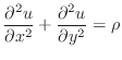 |
(1) |
where  is the unknown function and
  is a given function. Boundary
conditions are necessary, and we will
be considering Dirichlet boundary conditions, i.e.,
is a given function. Boundary
conditions are necessary, and we will
be considering Dirichlet boundary conditions, i.e.,  at all
boundary points.
at all
boundary points.
Suppose that the unit square
![$ [0,1]\times[0,1]$](img7.png) is broken into
is broken into
 smaller, nonoverlapping squares, each of side
  . Each
of these small squares will be called ``elements'' and their corner
points will be called ``nodes.'' The combination of all elements
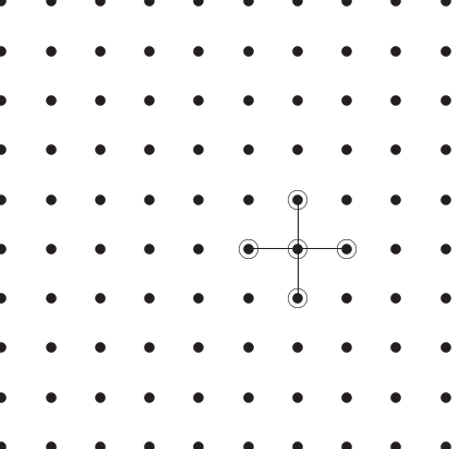
making up the unit square will be called a ``mesh.'' An example
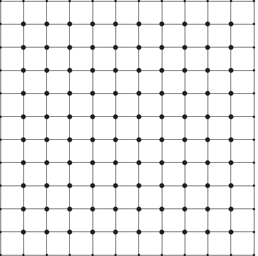
of a mesh is shown in Figure 1.
. Each
of these small squares will be called ``elements'' and their corner
points will be called ``nodes.'' The combination of all elements
making up the unit square will be called a ``mesh.'' An example
of a mesh is shown in Figure 1.
Figure 1:
A sample mesh, with interior nodes indicated by larger dots
and boundary nodes by smaller ones.
 |
The nodes in Figure 1 have coordinates  given by
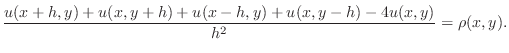
You will be generating the matrix associated with the Poisson equation
during this lab, using one of the simplest discretizations of this
equation, based on the finite difference expression for a second
derivative
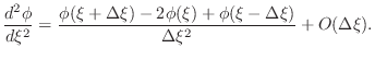 |
(3) |
Using (3) twice, once for
 and once for
  , in
(1) at a mesh node
yields the expression
, in
(1) at a mesh node
yields the expression
Denoting the point
as the ``center'' point, the point
 as the ``right'' point,
 as the ``left'' point,
 as the ``above'' point, and
 as the ``below'' point yields the expression
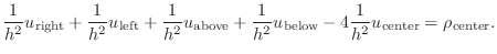 |
(4) |
Some authors denote these five points as ``center'', ``north'',
``east'', ``south'', and ``west'', referring to the compass directions.
The matrix equation (system of equations) can be generated from
(4) by numbering the nodes in some way and forming a
vector from all the nodal values of
. Then, (4)
represents one row of a matrix equation
 .
It is immediate that there are at most five non-zero terms in each row
of the matrix
.
It is immediate that there are at most five non-zero terms in each row
of the matrix  , no matter what the size of
. The diagonal
term is
, no matter what the size of
. The diagonal
term is
 , the other four, if present, are each equal to
 , and all remaining terms are zero. We will be
constructing such a matrix in Matlab during this lab.
, and all remaining terms are zero. We will be
constructing such a matrix in Matlab during this lab.
The equation in the form (4) yields the
``stencil'' of the differential
matrix, and is sometimes illustrated graphically as in Figure
2 below. Other stencils are possible and
are associated with other difference schemes.
Figure 2:
A sample mesh showing interior points and indicating
a five-point Poisson equation stencil.
 |
In order to construct matrices arising from the Poisson differential
equation, it is necessary to give each node at which a solution
is desired a number. We will be considering only the case of
Dirichlet boundary conditions (
at all boundary points),
so we are only interested in interior
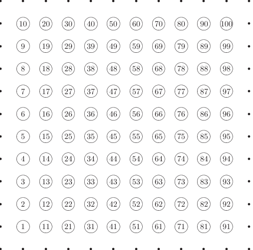
nodes illustrated in Figure 1. These nodes will
be counted consecutively, starting with 1 on the lower left and increasing
up and to the right to 100 at the upper right, as illustrated in
Figure 3. This is just one possible way of numbering
nodes, and many other ways are often used. Changing the numbering
changes the rows and columns of the resulting matrix.
Figure 3:
Node numbering
 |
-
- Exercise 1:
- Write a script m-file, named meshplot.m that, for
N=10, generates two vectors, x(1:N^2)
and y(1:N^2) so that the points with coordinates
(x(n),y(n)) for n=1,...,N^2 are the
interior node points illustrated in Figures 1,
2
and 3 and defined in (2).
The following outline employs two loops on j and k
rather than a single loop on n. The double loop approach
leads to somewhat simpler code.
N=10;
h=1/(N+1);
n=0;
% initialize x and y as column vectors
x=zeros(N^2,1);
y=zeros(N^2,1);
for j=1:N
  for k=1:N
    % xNode and yNode should be between 0 and 1
    xNode=???
    yNode=???
    n=n+1;
    x(n)=xNode;
    y(n)=yNode;
  end
end
plot(x,y,'o');
- Send me your plot. It should look similar to Figure
2, but without the stencil.
- The following function m-file will print,
for n given and N=10, the index (subscript) value
associated with the point immediately above the given point,
or the word ``none'' if there is no such point.
function tests(n)
% function tests(n) prints index numbers of points near the
% one numbered n

% your name and the date.

N=10;
if mod(n,N)~=0
  nAbove=n+1
else
  nAbove='none'
end
Copy this code to a file named tests.m and
test it by applying it with n=75
to find the number of the point above the one numbered 75. Test it
also for n=80 to see that there is no point above the one numbered 80.
- Add similar code to tests.m
to print the index nBelow of the
point immediately below the given point. Use it to find the
number of the point below the one numbered 75, and also apply it to a
point that has no interior point below it.
- Add similar code to tests.m
to print the index nLeft of the
point immediately to the left of the given point. Use it to find
the number of the point to the left of the one numbered 75, and
also apply it to a point that has no interior point to its left.
- Add similar code to tests.m
to print the index nRight of the
point immediately to the right of the given point. Use it to find
the number of the point to the right of the one numbered 75, and also
apply it to a point that has no interior point to its right.
You are now ready to construct a matrix  derived from the
Poisson equation with Dirichlet boundary conditions on a uniform
mesh. In this lab we are considering only one of the infinitely
many possibilities for such a matrix. The matrix
defined
above turns out to be negative definite, so the matrix
we will use in this lab is its negative,
derived from the
Poisson equation with Dirichlet boundary conditions on a uniform
mesh. In this lab we are considering only one of the infinitely
many possibilities for such a matrix. The matrix
defined
above turns out to be negative definite, so the matrix
we will use in this lab is its negative, 
-
- Exercise 2:
- Recall that there are no more than five non-zero entries per row
in the matrix
and that they are the values
 , and
, and  repeated
no more than four times. (Recall that
is the negative of the matrix
above.) Use the following skeleton, and your work from the
previous exercise, to write a function m-file to generate the matrix A.
repeated
no more than four times. (Recall that
is the negative of the matrix
above.) Use the following skeleton, and your work from the
previous exercise, to write a function m-file to generate the matrix A.
function A=poissonmatrix(N)
% A=poissonmatrix(N)
% more comments

% your name and the date

h=1/(N+1);
A=zeros(N^2,N^2);
for n=1:N^2
  % center point value
  A(n,n)    =4/h^2;

  % "above" point value
  if mod(n,N)~=0
    nAbove=n+1;
    A(n,nAbove)=-1/h^2;
  end

  % "below" point value
  if ???
    nBelow= ???;
    A(n,nBelow)=-1/h^2;
  end

  % "left" point value
  if ???
    nLeft= ???;
    A(n,nLeft)=-1/h^2;
  end

  % "right" point value
  if ???
    nRight= ???;
    A(n,nRight)=-1/h^2;
  end

end
In the following parts of the exercise, take N=10 and
A=poissonmatrix(N).
- It may not be obvious from our construction, but the matrix
A is symmetric. Consider A(ell,m) for
ell=n and m=nBelow, and also for ell=nBelow
and m=n (n is ``above'' nBelow).
Think about it.
Check that norm(A-A','fro') is essentially zero.
Debugging hint: If it is not zero, follow these instructions
to fix your poissonmatrix function.
- Set nonSymm=A-A', and
choose one set of indices ell,m for which nonSymm
is not zero. You can use the variable browser (double-click on
nonSymm in the ``variables'' pane) or the max
function in the following way:
  [rowvals]=max(nonSymm);
  [colval,m]=max(rowvals);
  [maxval,ell]=max(nonSymm(:,m));
- Look at A(ell,m) and A(m,ell). The most
likely case is that one of these is zero and the other is not.
Use your tests.m code to check which of them should be
non-zero, and then look to see why the other is not.
- It is not likely that A(ell,m) and A(m,ell)
are both non-zero but disagree because all non-zero, non-diagonal
entries are equal to -1/h^2. Check these values.
- The Gershgorin circle theorem (see, for example, your class notes, Quarteroni, Sacco and Saleri, or the interesting Wikipedia article
http://en.wikipedia.org/wiki/Gershgorin_circle_theorem)
says that the eigenvalues of a matrix
are contained in the union
of the disks in the complex plane centered at the points
 , and having radii
 .
By this theorem, our matrix A is non-negative definite.
A proof based on irreducible diagonal dominance exists,
showing that A is positive definite.
For a test vector v=rand(100,1), compute v'*A*v.
This quantity should be positive. If it is not, fix your
poissonmatrix function.
.
By this theorem, our matrix A is non-negative definite.
A proof based on irreducible diagonal dominance exists,
showing that A is positive definite.
For a test vector v=rand(100,1), compute v'*A*v.
This quantity should be positive. If it is not, fix your
poissonmatrix function.
- Positive definite matrices must have positive determinants.
Check that det(A) is positive. If it is not, fix your
poissonmatrix function.
- As in
Lab 5, Exercise 8,
a simple calculation shows that the functions
are eigenfunctions of the Dirichlet problem for Poisson's equation
on the unit square for each choice of  and
and  , with
eigenvalues
, with
eigenvalues
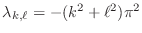 . It turns out
that, for each value of k and ell, the vector
E=sin(k*pi*x).*sin(ell*pi*y) is also an eigenvector
of the matrix A, where x and y are the
vectors from Exercise 1. The eigenvalue is
L=2*(2-cos(k*pi*h)-cos(ell*pi*h))/h^2,
where h=y(2)-y(1).
Choose k=1 and ell=2. What is L and,
for aid in grading your work, E(10)?
(E(10) should be negative and less than 1 in absolute value).
Show by computation that L*E=A*E, up to roundoff. If this is not true for
your matrix A, go back and fix poissonmatrix.
. It turns out
that, for each value of k and ell, the vector
E=sin(k*pi*x).*sin(ell*pi*y) is also an eigenvector
of the matrix A, where x and y are the
vectors from Exercise 1. The eigenvalue is
L=2*(2-cos(k*pi*h)-cos(ell*pi*h))/h^2,
where h=y(2)-y(1).
Choose k=1 and ell=2. What is L and,
for aid in grading your work, E(10)?
(E(10) should be negative and less than 1 in absolute value).
Show by computation that L*E=A*E, up to roundoff. If this is not true for
your matrix A, go back and fix poissonmatrix.
- It can be shown that A is an ``M-matrix'' (see,
Quarteroni, Sacco, and Saleri, or
Varga, Matrix Iterative Analysis), or the Wikipedia article
http://en.wikipedia.org/wiki/M-matrix)
because
the off-diagonal entries are all non-positive and
the diagonal entry meets or exceeds the negative of the sum of the off-diagonal
entries. It turns
out that M-matrices have inverses all of whose entries are
strictly positive. Use Matlab's inv
function to find the inverse of A and show that its smallest
entry (and hence each entry) is positive. (It might be small, but
it must be positive.)
- Finally, you can check your construction against Matlab itself.
The Matlab function gallery('poisson',N) returns a matrix
that is h^2*A. Compute
norm(gallery('poisson',N)/h^2-A,'fro') to see if it is
essentially
zero. (Note: The gallery function returns the
Poisson matrix in a special compressed form that is different from
the usual form and also not the same as the one discussed later
in this lab.) If this test fails, fix poissonmatrix.
You now have a first good matrix to use for the study of the conjugate
gradient iteration in the following section. In the following
exercise you will generate another.
-
- Exercise 3:
- Copy your poissonmatrix.m to another one called
anothermatrix.m (or use ``Save As'' on the ``File'' menu.)
- Modify the comments and some statements in the following way:
    A(n,n)     = 8*n+2*N+2;
    A(n,nAbove)=-2*n-1;
    A(n,nBelow)=-2*n+1;
    A(n,nLeft) =-2*n+N;
    A(n,nRight)=-2*n-N;
This matrix has the same structure as that from poissonmatrix
but the values are different.
- This matrix is also symmetric. Check that, for N=12,
norm(A-A','fro') is essentially zero. Debug hint:
If this norm is not essentially zero for N=12, but
is essentially zero for N=10, then you have the
number 10 coded in your function somewhere. Try searching for ``10''.
(If you have that error in anothermatrix.m you probably
have the same error in poissonmatrix.m.)
- This matrix is positive definite, just as the Poisson matrix is.
For N=12 and one test vector v=rand(N^2,1);
check that v'*A*v is positive.
- Plot the structure of the matrices and see they are the same.
First, examine the structure of poissonmatrix with the commands
spy(poissonmatrix(12),'b*');  % blue spots
hold on
Next, see that anothermatrix has non-zeros everywhere
poissonmatrix does by overlaying its plot on top of the previous.
spy(anothermatrix(12),'y*'); % yellow spots cover all blue
Finally, confirm that anothermatrix has no new non-zeros by
overlaying the plot of poissonmatrix.
spy(poissonmatrix(12),'r*'); % red spots cover all yellow
Please include this plot with your summary.
- To help me confirm that your code is correct,
what is the result of the following calculation?
N=15;
A=anothermatrix(N);
x=((1:N^2).^2)';
sum(A*x)
The conjugate gradient algorithm
The conjugate gradient method is an important iterative method
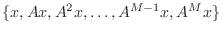
and one of the earliest examples of methods based on Krylov spaces.
Given a matrix
and a vector  , the space
spanned by the set
, the space
spanned by the set
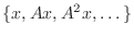 is called a
Krylov space.
is called a
Krylov space.
One very important point to remember about the
conjugate gradient method (and other Krylov methods) is that
only the matrix-vector product is required. One can
write and debug the method using ordinary matrix arithmetic
and then apply it using other storage methods, such as the
compact matrix storage used below.
A second very important point to remember is that the conjugate
gradient algorithm requires the matrix to be positive definite.
You will note that the algorithm below contains a step with
 in the denominator. This quantity is
guaranteed to be nonzero only if
is positive (or negative) definite.
If
is negative definite, multiply the equation through by (-1)
as we have done with the Poisson equation.
in the denominator. This quantity is
guaranteed to be nonzero only if
is positive (or negative) definite.
If
is negative definite, multiply the equation through by (-1)
as we have done with the Poisson equation.
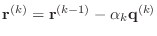
The conjugate gradient algorithm can be described in the following way.
Starting with an initial guess vector
 ,
,
-
- For
-
- if
 is zero, stop: the solution has been found.
- if
is 1
-

- else
-
-

- end
-

-
- if
 , stop:
is not positive definite
, stop:
is not positive definite
-
-
-
- end
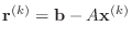
In this description, the vectors
 are the ''residuals.''
There are many alternative ways of expressing the conjugate gradient
algorithm. This expression is equivalent to most of the others.
(Two of the ``if'' tests guard against dividing by zero.)
are the ''residuals.''
There are many alternative ways of expressing the conjugate gradient
algorithm. This expression is equivalent to most of the others.
(Two of the ``if'' tests guard against dividing by zero.)
In the following exercise you will first write a function to
perform the conjugate gradient algorithm,
You will test it without using hand calculations.
-
- Exercise 4:
- Write a function m-file named cgm.m with signature
function x=cgm(A,b,x,m)
% x=cgm(A,b,x,m)
% more comments

% your name and the date
that performs m iterations of the conjugate gradient
algorithm for the problem A*y=b, with starting vector x.
Do not create vectors for the variables  ,
,  , and
, and
 , instead use simple Matlab scalars alpha for
,
beta for
, rhoKm1 for
, and
rhoKm2 for
, instead use simple Matlab scalars alpha for
,
beta for
, rhoKm1 for
, and
rhoKm2 for
 .
Similarly, denote the vectors
,
.
Similarly, denote the vectors
,
 ,
,
 , and
, and
 by the Matlab variables
r, p, q, and x, respectively.
For example, part of your loop might look like
by the Matlab variables
r, p, q, and x, respectively.
For example, part of your loop might look like
rhoKm1=0;
for k=1:m
  rhoKm2=rhoKm1;
  rhoKm1=dot(r,r);
  ???
  r=r-alpha*q;
end
- Use N=5, b=(1:N^2)',
A=poissonmatrix(N), xExact=A\b.
Use a perturbed value near the exact
solution x=xExact+sqrt(eps)*rand(N^2,1) as
initial guess, and take ten
steps. Call the result y. You should get that
norm(y-xExact) is
much smaller than norm(x-xExact).
(If you cannot converge when you start near
the exact solution, you will never converge!)
- Note 1: If your result
is not small, look at your code.
should be very small,
and
 should be larger than
, and
should also be very small. The resulting
should be larger than
, and
should also be very small. The resulting
 should be very small.
- Note 2: The choice sqrt(eps) is a good
choice for a small but nontrivial number.
- If
 the set of vectors
 must be linearly dependent because there are more vectors than
the dimension of the space. Consequently, the conjugate gradient algorithm
terminates after M=N^2 steps on an
matrix.
As a second test, choose N=5, xExact=rand(N^2,1) and
A= poissonmatrix(N). Set b=A*xExact and then use
cgm, starting from the zero vector, to solve the system
in N^2 steps. If you call your solution x, show that
norm(x-xExact)/norm(xExact) is essentially zero.
must be linearly dependent because there are more vectors than
the dimension of the space. Consequently, the conjugate gradient algorithm
terminates after M=N^2 steps on an
matrix.
As a second test, choose N=5, xExact=rand(N^2,1) and
A= poissonmatrix(N). Set b=A*xExact and then use
cgm, starting from the zero vector, to solve the system
in N^2 steps. If you call your solution x, show that
norm(x-xExact)/norm(xExact) is essentially zero.
- You know that your routine solves a system of size M=N^2 in
M steps. Choose N=31;xExact=(1:N^2)';,
the matrix A=poissonmatrix(N), and
b=A*xExact. How close would the solution x calculated
using cgm on A be if
you started from the zero vector and took only one hundred steps? (Use
the relative 2-norm.)
The point of the last part of the previous exercise is that there
is no need to iterate to the theoretical limit. Conjugate
gradients serves quite well as an iterative method, especially
for large systems. Regarding it as an interative method, however,
requires some way of deciding when to stop before doing  iterations on an
  matrix. Assuming that
 a reasonable stopping criterion is when the relative residual error
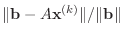 is small.
(If
is small.
(If
 , then
  is trivial, and so is the solution.)
Without an estimate of the condition number of
, this criterion
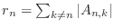
does not bound the solution error, but it will do for our purpose. A simple
induction argument will show that
is trivial, and so is the solution.)
Without an estimate of the condition number of
, this criterion
does not bound the solution error, but it will do for our purpose. A simple
induction argument will show that
 ,
so it is not necessary to perform a matrix-vector multiplication
to determine whether or not to stop the iteration. Conveniently,
the quantity
that is computed at the beginning
of the loop is the square of the norm of
,
so it is not necessary to perform a matrix-vector multiplication
to determine whether or not to stop the iteration. Conveniently,
the quantity
that is computed at the beginning
of the loop is the square of the norm of
 , so
the iteration can be terminated without any extra calculation.
, so
the iteration can be terminated without any extra calculation.
In the following exercise, you will modify your cgm.m
file by eliminating the parameter m in favor of a
specified tolerance on the relative residual.
-
- Exercise 5:
- Make a copy of your cgm.m function and call it
cg.m. Change its name on the signature line, but
leave the parameter m for the moment. Modify it by
computing
 and calling the value normBsquare, before the
loop starts. Then, temporarily add
a statement following the computation of rhoKm1
to compute the quantity relativeResidual=sqrt(rhoKm1/normBsquare).
Follow it with the commands
semilogy(k,relativeResidual,'*');hold on; so that you can watch
the progression of the relative residual.
and calling the value normBsquare, before the
loop starts. Then, temporarily add
a statement following the computation of rhoKm1
to compute the quantity relativeResidual=sqrt(rhoKm1/normBsquare).
Follow it with the commands
semilogy(k,relativeResidual,'*');hold on; so that you can watch
the progression of the relative residual.
- As in the last part of the previous exercise, choose
N=31;xExact=(1:N^2)', the matrix A=poissonmatrix(N),
and b=A*xExact. Run it for 200 iterations starting from
zeros(N^2,1). You will have to
use the command hold off after the function is done. Please
include the plot with your summary. You should observe uneven but
rapid convergence to a small value long before
 (many, many fewer
than
(many, many fewer
than  ) iterations.
Estimate from the plot how many iterations it would take to meet
a convergence criterion of
) iterations.
Estimate from the plot how many iterations it would take to meet
a convergence criterion of  .
.
- Change the signature of your cg function to
[x,k]=cg(A,b,x,tolerance)
so that m is no longer input. Replace the value m in
the for statement with size(A,1) because you know
convergence should
be reached at that point. Compute
targetValue=tolerance^2*normBsquare.
Replace the semilogy plot with the exit commands
  if rhoKm1 < targetValue
    return
  end
There is no longer any need for relativeResidual or the plot.
- As in the last part of the previous exercise, choose
N=31;xExact=(1:N^2)', the matrix A=poissonmatrix(N),
and b=A*xExact. Start from zeros(N^2,1).
Run your changed cg function with a tolerance of
1.0e-10. How many iterations does it take? What is the true
error (norm(x-xExact)/norm(xExact))? Run it with a tolerance
of 1.0e-12. How many iterations does it take this time? What is the
true error?
- To see how another matrix might behave, choose N=31,
xExact=(1:N^2)', the matrix A=anothermatrix(N),
and b=A*xExact. How many iterations does it take to
reach a tolerance of 1.e-10? What is the true error?
As you can see, the stopping criterion you have programmed is OK for
some matrices, but not all that reliable. Better stopping criteria
are available, but there is no generally accepted ``best'' one.
We now leave the discussion of stopping criteria to consider
alternative storage strategies.
In the following section, you will turn to an example of
an efficient storage schemes for some sparse matrices.
Compact storage
A matrix A generated by either poissonmatrix or
anothermatrix has only five
non-zero entries in each row. When numbered as above, it has exactly five
non-zero diagonals: the main diagonal, the super- and
sub-diagonals, and the two diagonals that are N columns
away from the main diagonal. All other entries are zero. It
is prudent to store A in a much more compact form by
storing only the diagonals and none of the other zeros. Further,
A is symmetric, so it is only necessary to store three
of the five diagonals. While not all matrices have such a nice
and regular structure as these, it is very common to encounter
matrices that are sparse (mostly zero entries). In the exercises
below, you will be using a very simple compact storage, based on
diagonals, but you will get a flavor of how more general compact
storage methods can be used.
Remark: Since an  matrix is rectangular,
there will still be some extraneous zeros in this ``by diagonals''
storage strategy.
matrix is rectangular,
there will still be some extraneous zeros in this ``by diagonals''
storage strategy.
Remark: Since poissonmatrix contains
only two different numbers, it can be stored in an even more
efficient manner, but we will not be taking advantage of this
strategy in this lab.
Since there are only three non-zero diagonals, you will see how
to use a
rectangular matrix to store a matrix that would
be
if ordinary storage were used. Further, since the
matrices from poissonmatrix and anothermatrix
are always
 , we will only consider the case that
 . The ``main diagonal'' is the one consisting of entries
 , the ``superdiagonal'' is the one consisting of entries
 and non-zero diagonal farthest from the main diagonal
consists of entries
and non-zero diagonal farthest from the main diagonal
consists of entries  , where
  . For the purpose
of this lab, we will call the latter diagonal the ``far diagonal.''
. For the purpose
of this lab, we will call the latter diagonal the ``far diagonal.''
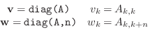
Conveniently,
Matlab provides a function to extract these diagonals from an
ordinary square matrix and to construct an ordinary square matrix
from diagonals. It is called diag and it works in
the following way. Assume that
is a square matrix
with entries
 . Then
where n can be negative,
so diag returns a column vector whose elements are diagonal entries
of a matrix. The same diag function also performs the reverse
operation.
Given a vector
 with entries
  , then
A=diag(v,n)
returns a matrix A consisting of all zeros except
that
, then
A=diag(v,n)
returns a matrix A consisting of all zeros except
that
 , for
, for
 . You must
be careful to have the lengths of the diagonals and vectors correct.
. You must
be careful to have the lengths of the diagonals and vectors correct.
In the following exercise, you will rewrite poissonmatrix
and anothermatrix to use storage by diagonals.
-
- Exercise 6:
- Copy your anothermatrix.m file to one called
anotherdiags.m (or use ``Save as''). Change the
name on the signature line and change the comments to indicate
the resulting matrix will be stored by diagonals.
- The superdiagonal corresponds to nAbove and
the far diagonal corresponds to nRight. Modify
the code so that the matrix A has three columns,
the first column is the main diagonal, the second column
is the superdiagonal, and the third column is the far diagonal.
The superdiagonal will have one fewer entry than the main diagonal,
so leave a zero as its last entry. The far diagonal will have N fewer
entries than the main diagonals, so leave zeros in the last
N positions.
- Your function should pass the following test
N=10;
A=anothermatrix(N);
Adiags=anotherdiags(N);
size(Adiags,2)-3                      % should be zero
norm(Adiags(:,1)-diag(A))             % should be zero
norm(Adiags((1:N^2-1),2)-diag(A,1))   % should be zero
norm(Adiags((1:N^2-N),3)-diag(A,N))   % should be zero
If not all four numbers are zero, fix your code. If you are debugging,
it is easier to use N=3.
- Repeat the steps to write poissondiags.m by starting
from poissonmatrix.m. Be sure to test your work.
If you look at the conjugate gradient algorithm, you will see that
the algorithm only made use of the matrix is to multiply the matrix by a
vector. If we plan to store a matrix by diagonals, we need to
write a special ``multiplication by diagonals'' function.
-
- Exercise 7:
- Start off a function m-file named multdiags.m
in the following way
function y=multdiags(A,x)
% y=multdiags(A,x)
% more comments

% your name and the date

M=size(A,1);
N=round(sqrt(M));
if M~=N^2
  error('multdiags: matrix size is not a squared integer.')
end
if size(A,2) ~=3
  error('multdiags: matrix does not have 3 columns.')
end

% the diagonal product
y=A(:,1).*x;
% the superdiagonal product
for k=1:M-1
  y(k)=y(k)+A(k,2)*x(k+1);
end
% the subdiagonal product
???
% the far diagonal product
???
% the far subdiagonal product
???
- Fill in the three groups of lines indicated by ???.
Hint: To see the logic, think of the product B*x,
where B is all zeros except for one of the diagonals.
- Choose N=3, x=ones(9,1), and compare
the results using multdiags to multiply anotherdiags
by x with the results of an ordinary multiplication by
the matrix from anothermatrix. The results should
be the same.
Debugging hints:
- All the components of x
are =1 in this case, so the only places your code might be wrong
in this test are in the subscripts of A.
- Look at the rows one at a time. Row k
of the full matrix product for B=anothermatrix(3) can be written as
x=ones(9,1);
B(k,:)*x
- For k=1 the product is
B(1,1)*x(1)+B(1,2)*x(2)+B(1,4)*x(4)
Check that you have this correct.
- For k=2 the product is
B(2,1)*x(1)+B(2,2)*x(2)+B(2,3)*x(3)+B(2,5)*x(5)
(This product has only the subdiagonal term in it.)
Check that you have this correct and continue.
- Choose N=3, x=(10:18)', and compare
the results using multdiags to multiply anotherdiags
by x with the results of an ordinary multiplication by
the matrix from anothermatrix. The results should
be the same.
- Choose N=12, x=rand(N^2,1), and
compare the results using multdiags to multiply
anotherdiags by x with the results of an
ordinary multiplication by the matrix from anothermatrix.
The results should be the same.
Remark: It is generally true that componentwise
operations are faster than loops. The multdiags function
can be made to execute faster by replacing the loops with componentwise
operations. This sounds complicated, but there is an easy trick.
Consider the superdiagonal code:
% the superdiagonal product
for k=1:M-1
  y(k)=y(k)+A(k,2)*x(k+1);
end
Look carefully at the following code. It is equivalent, very similar
in appearance and will execute more quickly.
k=1:M-1;  % k is a vector!
y(k)=y(k)+A(k,2).*x(k+1);
Then manually replacing the vector k and eliminating it generates
the fastest code:
y(1:M-1)=y(1:M-1)+A(1:M-1,2).*x(2:M);
You are not required to make these changes for this lab, but you might
be interested in trying.
Conjugate gradient by diagonals
Now is the time to put conjugate gradients together with storage
by diagonals. This will allow you to handle much larger matrices
than using ordinary square storage.
-
- Exercise 8:
- Copy your cg.m file to cgdiags.m. Modify
each product of A times a vector to use multdiags.
There are only two products: one before the for loop and
one inside it. You do not need to change any other lines.
- Solve the same problem twice, once using anothermatrix
and cg and again using anotherdiags and cgdiags.
In each case, use N=3, b=ones(N^2,1),
tolerance=1e-10, and start from zeros(N^2,1).
You should get exactly the same number of iterations and exactly the
same answer in the two cases.
- Solve a larger problem twice, with N=10 and
b=rand(N^2,1). Again, you should get the same answer in
the same number of iterations.
- Construct a much larger problem to which you know the solution
using the following sample code
N=500;
xExact=rand(N^2,1);
Adiags=poissondiags(N);
b=multdiags(Adiags,xExact);
tic;[y,n]=cgdiags(Adiags,b,zeros(N^2,1),1.e-6);toc
How many iterations did it take? How much time did it take?
Debugging hint: If you get a memory error message,
``Out of memory. Type HELP MEMORY for your options,'' you most likely
are attempting to construct the full Poisson matrix using normal
storage, an impossible task (see the next exercise). Examine your
poissondiags.m code carefully with this in mind.
- You can compute the relative norm of the error because you
have both the computed and exact solutions. What is it?
How does it compare with the tolerance? Recall that the tolerance
is the relative residual norm and may result in the
error being either larger or smaller than the tolerance.
In the previous exercise, you saw that the conjugate gradient
works as well using storage by diagonals as using normal storage.
You also saw that you could solve a matrix of size
 , stored by diagonals. This matrix is actually quite
large, and you would not be able to even construct it, let
alone solve it by a direct method, using ordinary storage.
, stored by diagonals. This matrix is actually quite
large, and you would not be able to even construct it, let
alone solve it by a direct method, using ordinary storage.
-
- Exercise 9:
- Roughly, how many entries are in the Adiags from
the previous exercise?
If one number takes eight bytes, how many
bytes of central memory does Adiags take up?
- Roughly, what would the total size of poissonmatrix(N)
(for N=500) be? If one number takes eight bytes of central
memory, how many bytes of central memory would it take to store that
matrix? While the cost of RAM memory for PCs varies greatly,
use a price of about US$4 for 1GB of RAM memory (
 or roughly
  bytes). How much would it cost to purchase enough
memory to store that matrix? I recently purchased a computer for
$1400. Does your estimated cost for memory alone exceed the cost
of my computer?
bytes). How much would it cost to purchase enough
memory to store that matrix? I recently purchased a computer for
$1400. Does your estimated cost for memory alone exceed the cost
of my computer?
- In Lab 6, Exercise 2, you found that the time it takes
to solve a matrix equation using ordinary Gaußian elimination is
proportional to
 , where
is the size of the matrix.
I found it takes about
, where
is the size of the matrix.
I found it takes about  minute to solve a system of size
 .
Find
.
Find  so that
  holds.
- How long would it take to use Gaußian elimation to solve
a matrix equation using poissonmatrix(N) (N=500)?
Please convert your result from seconds to days. How does this
compare with the time it actually took to solve such a matrix equation
in the previous exercise?
-
- Exercise 10: Matlab has a built-in compact storage method for general sparse
matrices. It is called ``sparse storage,'' and it is a version
of ``compressed column storage.'' It is not difficult
to see how it works by looking at the following example. As you
saw above, the gallery('poisson',N) constructs a matrix
that is h^2 times the matrix from poissonmatrix.
- Use the following command to print out a sparse matrix
A=gallery('toeppen',8,1,2,3,4,5)
and you should be able to see how it is stored.
From what you just printed what do you think A(2,1),
A(3,2) and A(5,1) are?
- What are all the nonzero entries in column 4? What are all the
nonzero entries in row 4? Please report both indices and values in
your answer.
- Consider the full matrix
B=[ 1 0 0 2
    0 0 3 0
    0 4 0 0
    5 0 6 0];
If B were stored using Matlab's sparse storage method, what
would be the result of printing B (as you printed A).
Extra Credit: ICCG (8 points)
The conjugate gradient method has many advantages, but it can be
slow to converge, a disadvantage it shares with other Krylov-based
iterative methods. Since Krylov methods are perhaps the most widely-used
iterative methods, it is not surprising that there is a large effort
to devise ways to make them converge faster. The largest class of such
convergence-enhancing methods is called ``preconditioning'' and is
sometimes explained as solving the system
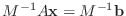 instead of
 , where
is a suitably chosen,
easily inverted matrix. More precisely, it solves
, where
is a suitably chosen,
easily inverted matrix. More precisely, it solves
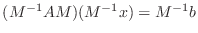 .
.
The preconditioned conjugate gradient algorithm can be described
in the following way.
Starting with an initial guess vector
,
-
- For
- Solve the system
 .
.
-
- if
is zero, stop: the solution has been found.
- if
is 1
-

- else
-
-
- end
-
-
- if
, stop:
is not positive definite
-
-
-
- end
In this form, the residuals
 can be shown to be
 -orthogonal, in contrast with the residuals being orthogonal
in the usual sense in the earlier, un-preconditioned, conjugate gradient
algorithm.
-orthogonal, in contrast with the residuals being orthogonal
in the usual sense in the earlier, un-preconditioned, conjugate gradient
algorithm.
One of the earliest effective preconditioners disovered was the
so-called ``incomplete Cholesky'' preconditioner. Recall that a
positive definite symmetric matrix
can always be factored as
 , where
  is an upper-triangular matrix with positive
diagonal entries. Although there are several different preconditioners
with the same name, the one that is easiest to describe and use here
is simply to take
is an upper-triangular matrix with positive
diagonal entries. Although there are several different preconditioners
with the same name, the one that is easiest to describe and use here
is simply to take
For sparse matrices
, this results in a upper triangular factor
 with the same sparsity pattern as
. If you
were using matrix storage by diagonals as in the exercises above, you
could store
using the same sort of three column matrix
that is used for the matrix
itself. Of course,
with the same sparsity pattern as
. If you
were using matrix storage by diagonals as in the exercises above, you
could store
using the same sort of three column matrix
that is used for the matrix
itself. Of course,
 . Choosing
 in
the preconditioned conjugate gradient results in the ``incomplete
Cholesky conjugate gradient'' method (ICCG).
in
the preconditioned conjugate gradient results in the ``incomplete
Cholesky conjugate gradient'' method (ICCG).
For large, sparse matrices
it is generally impossible to construct
the true Cholesky factor
, and, if you can construct it, it is
usually better to simply solve the system using it rather than some
iterative method. On the other hand, there are ways of producing
matrices
 that have the same sparsity pattern as
and perform as well as
. For our
purposes in this lab, we will be using
and seeing how
it improves convergence of the conjugate gradient method.
that have the same sparsity pattern as
and perform as well as
. For our
purposes in this lab, we will be using
and seeing how
it improves convergence of the conjugate gradient method.
-
- Exercise 11:
- Modify your cg.m m-file to precg.m with
signature
function [x,k]=precg(U,A,b,x,tolerance)
% [x,k]=precg(U,A,b,x,tolerance)
% more comments

% your name and the date
and where U is assumed to be an upper-triangular matrix,
not necessarily the Cholesky factor of A, and M=U'*U.
(Use Matlab's backslash operator twice, once for U'
and once for U. Be sure to use parentheses so that
Matlab does not misinterpret your formulæ.)
Change the convergence criterion so that dot(r,r)<targetValue
to be consistent with cg. Test it with
U being the identity matrix, with A=poissonmatrix(10),
the exact solution xExact=ones(100,1), b=A*xExact, and
starting from x=zeros(100,1) with tolerance=1.e-10.
You should get exactly the same values
for x and k as produced by cg.
- Look carefully at the algorithm above for the preconditioned
conjugate gradient. If
 and if
  ,
in symbols (not numbers), what are the values of
,
in symbols (not numbers), what are the values of
 ,
,
 ,
,  , and
, and  ? Your calculation should prove that
 at convergence.
- The Matlab chol(A) function returns the upper triangular
Cholesky factor. Using the following values
N=10;
xExact=ones(N^2,1); % exact solution
A=poissonmatrix(N);
b=A*xExact;         % right side vector
tolerance=1.e-10;
U=chol(A);          % Cholesky factor of A
x=zeros(N^2,1);
Use precg to solve this problem. Check that the value of
k is 2 at convergence, and that the solution is correct.
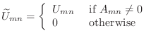
- The incomplete Cholesky factor,
, can be easily constructed
in Matlab with the following code.
U=chol(A);
U(find(A==0))=0;
(Or, equivalently, U(A==0)=0.)
Consider the system
starting from
for
given by anothermatrix(50)
and
 given as all ones and with a tolerance of 1.e-10.
Find the exact solution as xExact=A\b.
Compare the numbers of iterations
and true errors between the conjugate gradient and ICCG methods.
You should observe a significant reduction in the number of iterations
without loss of accuracy.
given as all ones and with a tolerance of 1.e-10.
Find the exact solution as xExact=A\b.
Compare the numbers of iterations
and true errors between the conjugate gradient and ICCG methods.
You should observe a significant reduction in the number of iterations
without loss of accuracy.
Note: If you measured the times for precg
and cg in the exercise, you might observe that there is little or no
improvement in running time for precg, despite the reduction
in number of iterations. If you try it with larger values of N
(for example, N=75), you will see more of an advantage, and
it will increase with increasing N. Alternatively, if you
implemented it using storage by diagonals as above, you would find
the advantage shows up for smaller values of N.
Back to MATH2071 page.
kimwong
2019-04-19