


Next: NMDA
Up: Glutamate
Previous: Glutamate
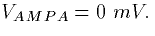
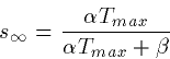
A simple first order kinetic model works
well for the fast excitatory AMPA receptor:
| 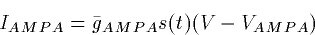 |
(3) |
| ![\begin{displaymath}
\frac{ds}{dt} = \alpha [T] (1-s) - \beta s\end{displaymath}](img30.gif) |
(4) |
where [T] is the concentration of transmitter given by
(2). The data taken from cortical cells is best fit by
setting 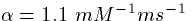 ,
, 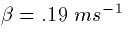 and
and
 If we suppose that that transmitter occurs in a
square pulse (not too bad an approximation), then the equation for s
is just linear with constant coefficents and can be solved. If the
transmitter is released at t=t0 and lasts until t=t1 then
If we suppose that that transmitter occurs in a
square pulse (not too bad an approximation), then the equation for s
is just linear with constant coefficents and can be solved. If the
transmitter is released at t=t0 and lasts until t=t1 then

where
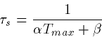
After the pulse turns off at t=t1,
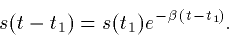
Thus, the synapse rises exponentially with a time constant  and decays with a time constant
  This simple form has
led many modelers to dispense with the differential equations
altogether and use the so-called ``alpha'' functions for s(t)
which have the
form
This simple form has
led many modelers to dispense with the differential equations
altogether and use the so-called ``alpha'' functions for s(t)
which have the
form

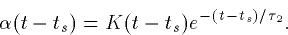
where ts is the time of the presynaptic spike (when the presynaptic
voltage crosses some set threshold),  is the rise time of the synapse (approximately
) and
is the rise time of the synapse (approximately
) and  is the decay of the synapse (approximately
 ). In particular, if the rise time is very fast, then
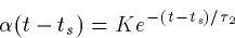
while if the decay and rise times are close,
The problem with using the so called ``alpha'' functions is that there
is some question what to do when there are multiple spikes.
Multiple spikes can either be added or the most recent
taken. This approach requires monitoring the presynaptic cells and
then setting/resetting the synaptic time-courses, s(t) for each
synapse.
This method of modeling has the advantage that no real dynamics must
be computed; once the synapse is set in motion, it follows the
prescribed time course. However, Destexhe et al show that using the
actual differential equations and the assumption that the pulse of
transmitter released is a square pulse, then the formulae above for
s(t) lead to a computationally efficient scheme for computing the
synaptic gates without having to keep track of all prior spikes. In my
opinion, the ``alpha'' functions are useful only for certain types of
exactly solvable models called integrate and fire models.
The AMPA synapses can be very fast. For example in some auditory
nuclei, they have submillisecond rise and decay times. In typical
cortical cells, the rise time is 0.4 to 0.8 milliseconds. Using the
above model with a transmitter concentration of 1 mM, the rise time
would be 1/(1.1+.19)=.8 msec. Decay is about 5 msec. As a final
note, AMPA receptors onto inhibitory interneurons are about twice as
fast in rise and fall times.
Next: NMDA
Up: Glutamate
Previous: Glutamate
G. Bard Ermentrout
2/12/1998