| HPS 0628 | Paradox | |
Back to doc list
The Infinite Lottery: the Chances
John D. Norton
Department of History and Philosophy of Science
University of Pittsburgh
http://www.pitt.edu/~jdnorton
What might it be to have a lottery that chooses among a countable infinity of outcomes? That question turns out to be a fertile source of problems and paradoxes. They are especially interesting to us here since they draw on many of the ideas that have been developed in earlier chapters.
• Should we extend the additivity of a probability measure from finite to countable additivity?
• What happens when problems like the Hilbert hotel become enmeshed in probabilistic system?
• What happens when we try to construct a chance system whose outcomes are probabilistically non-measurable and non-constructible?
These are the questions explored in this chapter and the next.
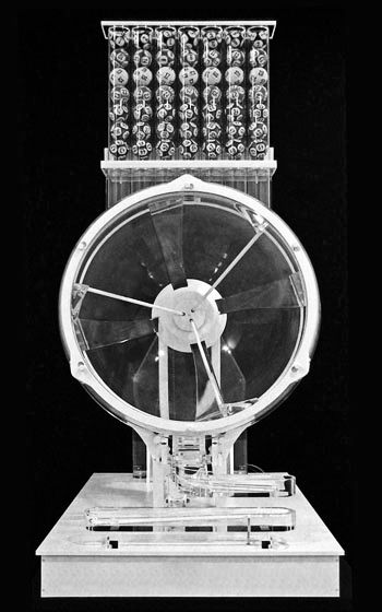
A traditional lottery or lotto machine is a mechanical device that makes a fair, that is, equal chance, selection among a finite number of outcomes. The machine may operate with paper tickets drawn by hand from a container; or a more sophisticated version has numbered balls that are tumbled in a barrel and then drawn off the bottom mechanically.
In the machine shown, the
numbered balls will be dropped from the overhead hopper into the barrel.
They are tumbled to mix them and then several are drawn off through a port
on the bottom.
Image source:
https://commons.wikimedia.org/wiki/File:TheBiLLeLottoBallMachine2012.jpg
An infinite lottery machine is essentially the same idea, but with an important extension. The machines chooses, fairly, among a countable infinity of balls, numbered 1, 2, 3, ...

There are two aspects to this infinite lottery machine to be pursued here.
First, there is an abstract problem in mathematics. What is it to choose fairly, that is, to choose with equal chance among a countable infinity of outcomes? The problem can be abstracted away from the mechanics of a lottery machine. It asks how can be distribute probabilities uniformly over an outcome set {1, 2, 3, 4, ...}
Second, is a mechanical problem. It will be discussed in the next chapter. To preview its concerns we can ask how we might go about constructing such a machine. There seems no realistic chance of actually building such a machine since handling an infinity of numbered balls lies outside normal human powers. But are these purely contingent problems? We would not expect any rope manufacturer to construct an infinitely long rope. But that is only because of the contingent problems such as a lack of infinite source materials and infinite time to build the rope. Or are the problems one of principle? Are they still beyond us if we allow extravagant idealizations such as supertasks? We would not expect a computing machine to be able to compute the last digit of the decimal expansion of π, even with idealization like supertasks, simply because there is no last digit. Is the construction of an infinite lottery machine similarly prohibited in principle?
What are the chances of different outcomes when we draw from an infinite lottery machine? We can write down a list of what we expect or would like to see in a probability measure that captures these chance properties:
Writing "1," "2," "3," ... for the outcome that a ball numbered 1, 2, 3, ... is drawn, we would like the following probabilistic results for finite sets of outcomes:
All single numbers have the same, very small probability. We shall call this very small probability ε:
P(1) = P(2) = P(3) = ... = ε
We would also like these probabilities to add up in the obvious way for finite sets of outcomes:
P(1 or 2 or 3) = P(1) + P(2) + P(3) = 3ε
Similar results apply to other finite sets.
For infinite sets of outcomes, we would like the following. We divide up the natural numbers into odd and even, thirds, quarters, and so on, we expect the probabilities of the sets so formed to have the probabilities 1/2, 1/3, 1/4, and so on. That is
P(odd) = P(1 or 3 or 5 or ...) = P(even) = P(2 or 4 or 6 or ...) = 1/2
so that these two rows of numbers each have the same probability of 1/2.
1
3 5 7 9 11 13 ...
2 4 6 8 10 12 14 ...
We also expect
1/3 = P(third-3: divisible by 3) = P(3 or 6 or 9 or
...)
= P(third-1: divisible by 3 plus 1) = P(4 or 7 or 10 or ...)
= P(third-2: divisible by 3 plus 2) = P(5 or 8 or 11 or ...)
so that these three rows of numbers each have the same probability of 1/3.
1
4 7 10 13 16 19 ...
2 5 8 11 14 17 20 ...
3 6 9 12 15 18 21 ...
As natural and simple as this list of wishes may be, they cannot all be satisfied by the probability measures commonly used. For they contradict the countable additivity of a probability measure. (The concept of countable additivity was explored in the earlier chapter, Additive Measures.)
The problem lies in the very small probability ε. If the probability measure is countably additive, ε must have contradictory properties. It can be neither equal to zero nor greater than zero. What results is a dilemma with no good choice.
If ε is some very small number greater than zero:
This choice fails since the computation of the probability of the whole outcome space leads to a contradiction:
P(1 or 2 or 3 or ...)
= P(1) + P(2) + P(3) + ...
= ε + ε + ε + ...
= ∞ x ε = ∞
This contradicts the unit normalization of the probability measure described in an earlier chapter. That is, a probability measure must assign unit probability to the whole outcome space
P(1 or 2 or 3 or ...) = 1
If ε =0:
This second choice produces a similar problem. For now we have
P(1 or 2 or 3 or ...)
= P(1) + P(2) + P(3) + ...
= ε + ε + ε + ... =
0 + 0 + 0 + ... = 0
This zero again contradicts the unit normalization of the probability measure.
A common solution follows the work of Bruno de Finetti. In it, we drop the countable additivity of the probability measure. For, as we have seen, the two summations above (with ε=0 and ε>0):
ε + ε + ε + ...
are infinite summations that require countable additivity. If we drop countable additivity, these summations are no longer allowed and the dilemma above cannot be formed.
In its place, we would simply continue with finite additivity only. Then we can assign ε = 0 without contradiction with the normalization of the probability distribution. For now we can only sum finitely many probabilities. The probability of any finite set of outcomes will be zero.
The zero probability of the individual outcomes no longer fixes the probability of infinite sets of outcomes. We are now free to assign unit probability to the full outcome set; and, if we like, probability 1/2 to each of the sets "even outcome" and "odd outcome." We now can have:
P(1) = P(2) = P(3) = ε = ... = 0
P(any number) = 1
P(even) = P(odd) = 1/2
Dropping countable additivity does seem awkward, given its importance in so many applications. One inducement is to note that countable additivity is violated if we look at frequencies in the countable outcome space.
For example, consider how we come to judge that half the numbers 1, 2, 3, 4, ... are even. The immediate problem is that all the numbers and the even numbers have the same infinite cardinality. Their ratio is ∞/∞, which has no definite value. We arrive at 1/2 by a more indirect method. The judgment that half the numbers are even is based on computing frequencies in a finite subset of numbers and taking a limit of an increasingly large subset of numbers. These sets might look like
1 2
3 4 5 6 7 8 9 10
(frequency even = 5/10=0.5)
1 2 3 4
5 6 7 8 9 10 11
(frequency even = 5/11=0.4545)
1 2 3 4
5 6 7 8 9 10 11 12
frequency even = 6/12=0.5)
1 2 3 4
5 6 7 8 9 10 11 12
13
frequency even = 6/13=0.4615)
...
As we make the subsets considered large, the frequency of even numbers approaches 1/2 arbitrarily closely. The limit frequency is 1/2.
If we apply the same reasoning to individual outcomes, we find that their limit frequencies are zero. Take the outcome 2, for example. In the same subsets as above, it has frequencies:
1 2
3 4 5 6 7 8 9 10
(frequency even = 1/10=0.1)
1 2 3
4 5 6 7 8 9 10
11
(frequency even = 1/11=0.0909)
1 2 3
4 5 6 7 8 9 10
11 12
frequency even = 1/12=0.0833)
1 2 3
4 5 6 7 8 9 10
11 12 13
frequency even = 1/13=0.0769)
...
As the subsets considered become arbitrarily large, the frequency of 2 comes arbitrarily close to zero. That is, the limit frequency is zero.
These limiting frequencies combined violate countable additivity. If we use countable additivity to compute the limit frequency of an even number, we recover a value of 0, not the 1/2 computed directly.
limit frequency (even number)
= limit frequency (2 or 4 or 6 or 8 or ...)
= limit frequency(2) + limit frequency (4) + limit frequency (8) + ...
= 0 + 0 + 0 + ... = 0
These results pertain so far to limiting frequencies computed in the specific way just sketched. IF--and this is a big IF--these limiting frequencies are identified with the probabilities, then we have recovered a finitely additive probability measure that is not countably additive.
Another response draws on the new mathematics of non-standard analysis. It adds new quantities to the familiar set of real numbers. In these new quantities, it possible to have infinitesimal quantities like ε that have the properties that escape the dilemma for ε laid out above. There we found that choosing either ε=0 or ε>0 led to a contradiction with the unit norm of a probability measure. Non-standard analysis, however, allows us to have an ε such that
ε > 0 and ε < any standard non-zero real number, like 1/2, 1/3, 1/4, ...
That is, this ε is greater than zero, but now "infinitesimally" small, that is, so small that we can longer add up infinitely many of them and recover an infinity that violates the unit norm of the probability measure.
That countably additivity must be dropped seems to me the right solution to the problems of an infinite lottery. However it seems to me that it is only a first step. A more complete solution requires that we also drop finite additivity.
The right way to respond to the difficulties of the
infinite lottery remains an open topic of debate in the philosophical
literature. The material presented in the remaining part of this chapter represents
my own approach to the infinite lottery problem. It is, I
believe, the correct approach. However you might find divergences in the
broader literature if you explore it.
To see why even finite additivity must go, we need to look more closely at what it means for the outcomes of an infinite lottery machine to be chosen fairly or without favor. That is a necessary condition for the proper operation of the machine. It is what will determine the notion of chance applicable to machines, like lottery machines.
The condition is easily stated in finite outcomes spaces with ordinary probabilistic randomizers such as tossed coins, rolled dice or spun roulette wheels. Each such device has number labels or other markings on them corresponding to their various outcomes.
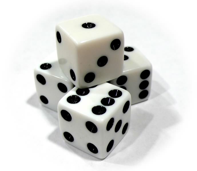

Imagine that we switch around the labels on these different devices. The faces labeled by the three and the six on a die, for example, might have their labels exchanged. If the device is fair, then the chances are unaffected by how we might have switched around the labels. We define:
Label independence: if a randomizing machine is fair, then the chances of an outcome or a set of outcomes are unaltered by any permutation of the labels marking the outcomes.
It is easy to see how this works if we imagine that a finite lottery machine chooses among six numbered balls by the spin of a pointer.

If the machine operation is fair then the chance of it drawing a six is unaffected by how we might rearrange the labels on the balls. We might switch neighboring pairs: 1↔2, 3↔4 and 5↔6:

Or we might rotate the labels around the dial: 1→2, 2→3, 3→4, 4→5, 5→6 and 6→1.

Or we might switch the labels on the left and right: 1↔6, 2↔5 and 3↔4:

None of these permutations affects the chances of each individual outcome. The same holds for the chances of sets of outcomes. The chance of an even outcome {2, 4, 6} is the same no matter how the labels are permuted.
Fairness would fail if the machine did not choose its outcomes with equal chances. Consider the alternative design of a randomizer below. If we assume that the pointer spins freely and ends up with equal chances in all directions, then this new machine does not assign equal chances to all the outcomes:

Balls numbered 1, 2 and 3 have a greater chance of selection that do balls numbered 4, 5 and 6.
To see that label independence would fail, imagine that we now permute labels according to 1 ↔ 6, 2 ↔ 5 and 3 ↔ 4. We arrive at:

Prior to the permutation we would have
Chance(1) > Chance(6)
Chance(2) > Chance(5)
Chance(3) > Chance(4)
and for the sets small = {1, 2, 3} and large = {4, 5, 6}
Chance (small) > Chance (large)
After the permutation, we have
Chance(1) < Chance(6)
Chance(2) < Chance(5)
Chance(3) < Chance(4)
Chance (small) < Chance (large)
Since the permutation has changed the chances of individual outcomes and sets of outcomes, the machine fails to respect label independence. We can conclude that it is not fair.
The notion of "switching
labels" here is one that must be implemented carefully. It must
be done such that:
• Every label is assigned to exactly one, possibly new location.
• No location is left without a label; or with more than one label.
This notion of switching is implemented by the mathematical notion of a "permutation." In set theory, a permutation is defined as a one-one mapping of a set back onto itself. If the labels are rearranged by a permtuation, the two conditions above are satisfied.
Let us now consider an infinite lottery machine. What is it for the machine to be fair? We now require that the machine satisfy label independence as a necessary part of its fair operation. At first, it will seem that the requirement of label independence produces results comparable with those produced for randomizers with finite outcome spaces. We will soon see, however, that here label independence requires a quite different notion of chance from the familiar one of probability theory.
To begin, consider the chances
of an odd outcome (1, 3, 5, ...) and an even outcome (2, 4, 6,
...). If we arrange the balls in two rows as shown, then we can see how a
permutation of the labels switches those balls that were initially labeled
odd with those that were initially labeled even:
(1↔2, 3↔4, 5↔6, 7↔8, ...)

Here is the same set of balls after the labels have
been switched:

Label independence requires that this permutation of the labels does not affect the chances of odd and even. That is, that the labels for 2, 4, 6, ... are now attached to different balls does not affect the chance of an even number, 2, 4, 6, ... Since these labels are attached to balls that formerly carried the odd number labels, it follows that the two outcomes of odd and even must have the same chance:
chance(even) = chance(odd)
We can give a similar analysis for three sets that divide up the numbers into thirds:
third-1 = {1, 4, 7, 10, 13, 16, ...}
third-2 = {2, 5, 8, 11, 14, 17, ...}
third-3 = {3, 6, 9, 12, 15, 18, ...}
The three sets are arranged in three rows. The
labels can be permuted as indicated among corresponding positions in the
three rows.

The labels on the second and third rows can be
exchanged, for example:

It follows that the sets associate with the second and third rows must have the same chance. Similar permutations allow us to infer that all three rows have the same chance:
chance(third-1) = chance(third-2) =
chance(third-3)
So far, these results are unremarkable. They have been recovered since we have chosen permutations that return unremarkable results. However none of these permutations have tested additivity. That will now change.
If these chances were to be represented by probabilities, we would have for the mutually exclusive outcomes third-1 and third-2 that
(additivity)
P(third-1 or third-2) = P(third-1) + P(third-2)
A different permutation shows that the applicable
notion of chance cannot be an additive probability measure. We
arrange the balls in just two rows. The first row has all the balls
labeled by third-1 and third-2. The second row has only the balls labeled
by third-3. This arrangement shows that there is a permutation that
switches the labels of (third-1 or third-2) with third-3:
1↔3, 2↔6, 4↔9, 5↔12, 7↔15, 8↔18, ...:

Label independence now tells us that the outcomes associated with these two rows have equal chances. That is:
chance(third-1 or third-2) = chance(third-3)
If we now recall that the chance of third-3 is the same as that of third-1 and third-2 individually, we arrive at
(additivity fails)
chance(third-1 or third-2) = chance(third-1) = chance(third-2)
It follows that the applicable notion of chance cannot be an additive probability measure. For an additive measure would require the chance of (third-1 or third-2) to be equal to the sum of chances of its two parts.
This demonstration of the failure of additivity depends essentially on the infinity of the lottery. If we tried to set up the same permutation over thirds in a finite lottery, the effort would fail. We would find that the first row (with third-1 and third-2) would be twice as long as the third row (with third-3). That means that a permutation switching labels on these two rows is impossible. In the attempt, half the balls in the first row would fail to be assigned number labels.
It is not too hard to see how these last results generalize.
To establish that two outcome sets have equal chances, all we need to be
able to do is to arrange them in two rows, so that we can see that a
permutation of labels is possible between them. This arrangement will be
possible for any outcome that:
• consists of a countable infinity of individual outcomes;
and
• its complement also consists of a countable infinity of
individual outcomes.
These are "infinite-co-infinite" sets of
outcomes.
For example, consider the set
tens = {10, 20, 30, 40, ...}
Its complement is everything that is not in tens:
tens-complement = {1, 2, 3, ..., 9, 11, 12, ..., 19, 21, 22, ...}
By arranging tens-complement in the first row and
tens in the second row, we can see that a permutation that switches their
labels is possible:

It follows that the outcomes in the two rows have equal chance:
chance(tens) = chance(tens-complement)
We arrive at similar results if we consider the set:
powers-of-ten = {10, 100, 1000, 10000, ...}
= {101, 102, 103, 104,...}
The requisite permutation is:

It follows that
chance(powers-of-ten) = chance(powers-of-ten-complement)
We could continue this pairing of countably infinite sets with their countably infinite complements. We arrive at a general result for chances of outcomes in an infinite lottery machine:
All infinite-co-infinite sets of outcomes in a countably infinite outcome space have the same chance.
This is a major result for the chances governing an infinite lottery, for most of the subsets of outcomes of an infinite lottery are infinite-co-infinite. (These sets are uncountably infinite. The remaining sets are only countably infinite.)
There is much more to say if we are to build up a complete theory of the chances of an infinite lottery. The logic needs to be extended to outcome sets that are finite; and to sets that are infinite with finite complements. However this much of the analysis displays the major difference between these infinite lottery chances and ordinary probabilistic chances.
One might imagine that these infinite lottery chances run into trouble when we consider frequencies. Are not the even numbers {2, 4, 6, 8, ...} one half of all the numbers? Should they not have a probability 1/2? Are not the multiples of three {3, 6, 9, ....} one third of the numbers, so they should have a probability of 1/3?
No. There is no simple fact that the even numbers are one half of all numbers. Rather, there is a more complicated fact concerning limits. We saw above that the frequency of even numbers approaches 1/2 as we consider larger, finite sets of numbers:
1 2
3 4 5 6 7 8 9 10
(frequency even = 5/10=0.5)
1 2 3 4
5 6 7 8 9 10 11
(frequency even = 5/11=0.4545)
1 2 3 4
5 6 7 8 9 10 11 12
frequency even = 6/12=0.5)
1 2 3 4
5 6 7 8 9 10 11 12
13
frequency even = 6/13=0.4615)
...
How can it be that the chance of an even number in an infinite lottery is anything other than 1/2?
The catch is that this judgment of 1/2 depends on the particular ordering of the numbers used in the calculations above. If we use a different ordering, we will get a different result. For example, we could use this ordering:
1 3 2
5 7 4 9 11 6 12
(frequency = 3/10 = 0.3)
1 3 2 5 7 4
9 11 6 12 13
(frequency = 3/11 = 0.2727)
1 3 2 5 7 4
9 11 6 12 13 8
(frequency = 4/12 = 0.3333
1 3 2 5 7 4
9 11 6 12 13 8 15
(frequency = 4/13 = 0.3077
1 3 2 5 7 4
9 11 6 12 13 8 15 17
(frequency = 4/14 = 0.2857)
1 3 2 5 7 4
9 11 6 12 13 8 15 17 10
(frequency = 5/15 = 0.3333)
...
With this alternative ordering, the frequency of even numbers will approach 1/3 arbitrarily closely as larger subsets are considered.
There is nothing intrinsically wrong with the assumption that these limits should be computed just using the natural ordering 1, 2, 3, 4, 5, .... However, nothing requires it. Indeed to require it is to add extra conditions to the infinite lottery machine specification. For now label indepedence alone no longer suffices to specify which outcome sets have equal chance. We must add in an extra condition about the limiting frequencies of the set. That is, we have changed the problem posed to another, more restrictive type of infinite lottery machine.
There is nothing wrong in principle with this different type of lottery machine. It is not, however, the lottery machine addressed in this chapter.
A potential problem with frequencies lies in another area. What happens if we run many infinite lotteries? Will we find that the frequencies of numbers drawn will vindicate the normal probabilities? Surely an even outcome is drawn half the time and and a multiple of three a third of the time.
The idea behind this last proposal depends on the
weak law of large numbers in probability theory, discussed in an earlier
chapter. It is, loosely speaking, that probabilities
are given by frequencies in large numbers of repeated trials. A
tossed coin has a probability of half of heads since, loosely speaking, we
will find roughly one half heads in many repeated tosses.
This associate of frequencies and probabilities holds only, "loosely speaking." A fuller statement of the weak law of large numbers says that the probability is arbitrarily high that the frequencies come arbitrarily close to the probabilities in repeated coin tosses.
That is, the association is itself a result within the probability calculus and can only be stated correctly as a result within the probability calculus.
So the question to ask now is whether there is a corresponding result within the theory of chance applicable to an infinite lottery machine. A full analysis of this question is given elsewhere (in the reference cited above: "Infinite Lottery Machines" Ch. 13 in John D. Norton, The Material Theory of Induction. BPSPopen, forthcoming.) In short, there is no corresponding result. Instead, it is possible to prove a result that says that chances do not favor any stabilization of frequencies.
Consider a large number--N--of infinite lottery
machines, each is run independently. We will track the frequencies of
outcomes in
ten = {10, 20, 30, 40, ...}
even = {2, 4, 6, 8, ...}
If the frequencies of various outcomes are to conform
with an analog of the weak law of large numbers, we would expect
for large N that:
It is very likely that a tenth of outcomes (N/10)
are in the set ten.
It is very likely that a half of the outcomes (N/2) are in the set even.
Instead, the result is that, among the N outcomes:
chance(0 in ten) = chance(0 in even)
chance(1 in ten) = chance(1 in even)
chance(2 in ten) = chance(2 in even)
...
chance(N/2 in ten) = chance(N/2 in even)
...
chance(N-1 in ten) = chance(N-1 in even)
chance(N in ten) = chance(N in even)
What this means is that we have no basis in the chances for expecting frequencies to behave as they would in a probabilistic system. If this set of chances somehow favors a massing of chances around N/2 for the even outcome, then the same massing happens for the tens outcomes. Or, if the set of chances favors a massing of chances around N/10 for the ten outcome, the same massing happens for the even outcomes. The massings of probabilities of the weak law of large numbers precludes the one massing applying to both of these outcomes. Whatever massings may arise here, they are not compatible with the sorts of frequencies needed for the probabilists' weak law of large numbers.
The chance notion developed here for an infinite lottery machine behaves rather differently from what we have come to expect. We arrived above at a failure of additivity:
(additivity fails)
chance(third-1 or third-2) = chance(third-1) = chance(third-2)
If we attach chance notions to betting behaviors, we might find this failure unsustainable. A bet on the outcome (third-1 or third-2) is surely more lucrative that a bet on either of its components. A bet on (third-1 or third-2) will win whenever one on third-1 does; and it will also win in cases where a bet on third-1 does not win. If we are to gauge the chances of outcomes by the attractiveness of bets, then it would seem that chance(third-1 or third-2) ought to be greater than chance(third-1).
This failure of additivity can be avoided, Matthew Parker has shown, if we are prepared to give up something natural elsewhere. It has been assumed that the chances of outcomes are always comparable:
Universal comparabiliity.
For any two outcomes, the first has greater, equal or lesser chance than
the second.
If we give up universal comparability, then the inferences that led to the failure of additivity can be blocked. A step in deriving the failure was the inference that
(third-1 or third-2) has the same chance as third-3
This step an be blocked if we posit:
The chances of disjoint outcome sets cannot be compared.
With this assumption made, Parker shows that we can build up a logic of chance based only on the notion of comparison:
"this outcome has greater/equal/lesser probability than that outcome."
In his logic, it turns out that
Chance(third-1 or third-2) is greater than
Chance(third-1)
Chance(third-1 or third-2) is greater than Chance(third-2)
In my view, this is a viable approach. The selection of whether it is better is to be made by deciding whether the loss of universal comparability is worth the gain of comparisons such as these last two.
The first chapter, "A Budget of Paradoxes," described the paradox of the two infinite lotteries. Here it is again:
Two infinite lottery machines will choose a number. The first, blue machine produces blue colored balls. The other, red machine produces red colored balls.

Will the red machine select
a number greater than the blue machine? It seems so. For when the blue
machine is run, it must select some ball. Imagine, for example, that the
number is 3. Then the red machine will select a number less than or equal
to 3 only in finitely many cases. It could choose 1 or 2 or 3. However
there are infinitely many ways the red machine can
choose a number greater than 3. It could choose 4, 5, 6, 7, 8, 9,
10, 11, ...

Since each ball has an equal chance of being selected, the chances are infinitely greater that the red machine will choose a number greater than 3.
This favoring of the red machine is true no matter which number the blue machine selects. If the blue machine selects 1,000,000,000, there are still infinitely more numbers the red machine can choose that are greater, but only finitely many that are fewer.
The operator of the blue machine is sure that the red machine will select a greater number.
The puzzle: The operator of the red machine carries out exactly the same inferences and concludes that the blue machine is sure to select a greater number.
Both cannot be correct.
The inference made from the perspective of the first, blue lottery machine is:
("Each to any")
If the first machine draws a 1, then it is very likely that the second
machine draws a greater number.
If the first machine draws a 2, then it is very likely that the second
machine draws a greater number.
If the first machine draws a 3, then it is very likely that the second
machine draws a greater number.
and so on for all the remaining numbers.
__________________________________________________
Therefore, it is very likely that the second machine draws a
greater number.
Call this inference "each to any," for convenience. The same inference is made from the perspective of the second, red machine. What results is:
It is very likely that the second machine draws a greater number; and it is very likely that first machine draws a greater number.
This is a contradiction since both cannot be very likely.
The resolution is that:
The "each to any" inference just sketched is a fallacy.
The easy way to see that it is a fallacy is show that it has true premises but a false conclusion. To do this we draw all the possible outcomes in an infinite array. Each pair of numbered balls represents one possible outcome of a single run on each of the machines. The diagonal shown collects all the cases in which the same number is drawn from both machines. In them, neither has the greater number. All cases not on the diagonal represent cases in which one machine has a greater number.

We can now represent the inferences made from the perspective of the first machine. Consider the cases in which the first machine draws a 3. All those cases are represented by the highlighted row:

Inspecting the row, we can see that there are only two cases in which the first, blue machine's 3 is greater than the number drawn by the second red machine (1 or 2). But there are infinitely many cases in which the second, red machine draws a number greater than 3.
This will be the case now matter which specific number is drawn by the first machine. Here is the figure corresponding to the first machine drawing a 4. The possible cases are found in a different row:

There are only 3 cases in which the first machine has drawn the greater number and infinitely many in which it has not.
Analogous facts obtain if we consider inferences made from the perspective of the second machine. If the second machine draws a 3, the figure is:

If the second machine draws of 4, the figure is:

In both cases, the second machine has drawn the greater number only in a few cases, but has drawn the smaller number in infinitely many.
What this shows is that premises of the "each to any" inference are true from both perspectives. Their truth is recovered from the figure.
We can also use the figure to test whether the conclusion of the "each to any" inference is true. The figure shows that the conclusion is false. The figure is symmetric about the diagonal in the drawings of the two machines. There is a one-one correspondence of outcomes in which the first lottery machine draws the greater number with those in which the second lottery machine draws the greater number. There is an equal chance that either lottery draws the greater number.

This analysis shows that the inference "each to any" above is a fallacy. It has true premises but a false conclusion. What might remain puzzling is how it could be a fallacy. To make the step from something being true for each to it being true for any seems secure. To say something is true for each looks like it it just the same thing as saying it is true for any. How can it go wrong?
??? each → any ???
The trouble is not due to some misuse of the terms "each" and "any." The trouble comes from an equivocation hidden in the inference. We are subtly changing the meaning of the term "very likely" in the transition from each to any. To see how that works, here is an example of an each to any inference in which true premises are attached to a true conclusion. We consider the balls drawn from the lottery machine that delivers only blue balls:
("Each to any")
If first machine draws a 1, then it is blue.
If first machine draws a 2, then it is blue.
If first machine draws a 3, then it is blue.
and so on for all the remaining numbers.
__________________________________________________
Therefore, any ball drawn from the machine is blue.
In this case, the meaning of the term blue is the same in each of the premises and in the conclusion. We pass without trouble from "each" to "any." This sameness of meaning, however, is lost in the each to any inference of the two lottery paradox:
("Each to any")
If the first machine draws a 1, then it is very
likely that the second machine draws a greater number.
If the first machine draws a 2, then it is very
likely that the second machine draws a greater number.
If the first machine draws a 3, then it is very
likely that the second machine draws a greater number.
and so on for all the remaining numbers.
__________________________________________________
Therefore, it is very likely
that the second machine draws a greater number.
Each of the terms "very likely" pertain to different outcome spaces:
The term very
likely in the first premise pertains to the reduced outcome space
in which the first machine has drawn a 1.
The term very likely in the second
premise pertains to the reduced outcome space in which the first machine
has drawn a 2.
The term very likely in the third
premise pertains to the reduced outcome space in which the first machine
has drawn a 3.
...and so on.
The term very likely in the conclusion, however, pertains to the full outcome space without any reduction that arises when a particular outcome of the draw on the first machine is known.
In short, the inference invites us to pass from premises, each employing different senses of "very likely," to a conclusion that employs the term "very likely" in a different sense again. If we proceed with the mistaken assumption that the meaning of the term "very likely" is the same in all instances, then we commit a fallacy of equivocation.
Another example of the fallacy of equivocation came up in an assignment:
A Jeep is better than nothing.
Nothing is better than a Cadillac.
Therefore, a Jeep is better than a Cadillac.
The term "nothing" has different meanings in each of the two premises.
The propositions in the "each to any" inference are really imprecise expressions for what are better presented as propositions within some definite theory of chance. Let us, for example, say that the theory of chance governing this case is that of a finitely additive probability measure "P(.)".
Consider the premise:
If the first machine draws a 3, then it is very likely that the second machine draws a greater number.
It is really a proposition in probability theory:
P(second machine number > first machine number | first machine draws 3) = 1
Similarly, consider the conclusion:
It is very likely that the second machine draws a greater number.
The conclusion is really a proposition in probability theory:
P(second machine number > first machine number) = 1
Whether this conclusion follows from the premises is not something that can be decided by looking at the imprecise statements of the "each to any" argument. They must be determined by the calculus governing the different probability spaces involved in the two propositions. The first is the space of:
P( . | first machine draws 3)
The second is the space of
P( . )
When we do the analysis, as suggested by the figures above, we find that the inference fails.
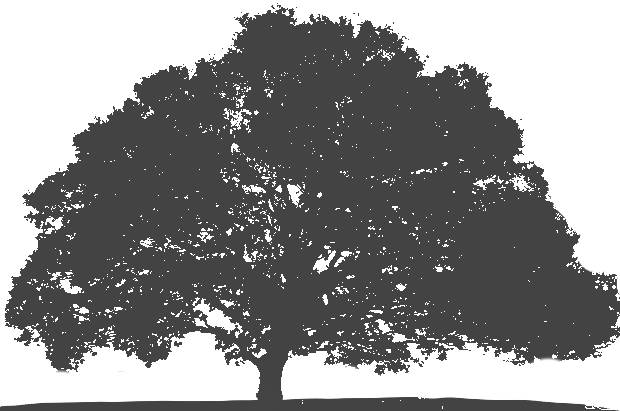
To get a sense of how a change in the outcome space can affect the truth of probabilistic statements, consider the proposition:
P(tree is taller than 5 feet) > 0.9
It is meaningless until we specify the outcome space. It would be true if the outcome space is the set of mature oak trees:
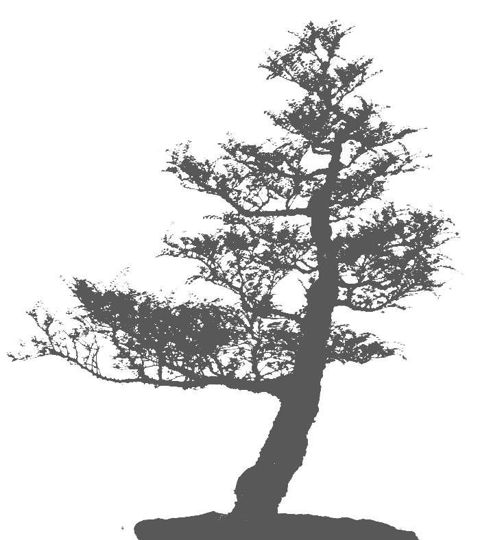
However it would be false if the outcome space is the set of bonsai trees:
The association of chance with probability, understood formally as an additive measure, is centuries old. Do we really need any other theoretical notion to deal with chance? Are not probabilities enough?
The chance notion described allows that the chance
of an outcome can equal that of its proper parts, such as
chance(third-1 or third-2) = chance(third-1) = chance(third-2)
Is this really admissible?
The criterion of label independence was illustrated and made plausible by examples in finite outcome spaces. Is that enough to assure us that it is a criterion suitable for use in infinite outcome spaces?
August 24, 28, December 8, 2021. April 20, 2023.
Copyright, John D. Norton