
| HPS 0628 | Paradox | |
Back to doc list
Paradoxes For Probability: Expectations
John D. Norton
Department of History and Philosophy of Science
University of Pittsburgh
http://www.pitt.edu/~jdnorton
The idea that expected value or expected utility is a good guide to the desirability of some option, such as a game, can lead us to paradoxical situations, when the expected utility is badly behaved. We shall see two cases with two different types of bad behavior. First is the St Petersburg Paradox (infinite expected utility). Second is the exchange paradox (ill-defined expected utility).
For a reminder of how expectations arise and are computed see Probability Theory Refresher
For many ordinary decision, expected value calculations can serve as a good guide. Choose the option with the greater expected value. They will tell you, for example, that there are no casino games worth playing extensively. For all of them have a negative expected value for each play. That is essential, since otherwise, the casinos could make no assured income. You may win or lose a little at the outset. However over the longer term, you fortune will bleed away as the negative expected values mount. Your loss is the casino's income. In summary:
Your choice:
Play a casino game: expected value is negative.
Do not play a casino game: expected value is zero.
However, there are many cases in which a favorable expectation is not enough to induce you to select that option. Here are several games, each with the same expected value per play.
| Game 1 | expected value +$1 | |
| Outcome | heads probability 1/2 |
tails probability 1/2 |
| net payoff | +$3 | -$1 |
| Game 10 | expected value +$1 | |
| Outcome | heads probability 1/2 |
tails probability 1/2 |
| net payoff | +$12 | -$10 |
| Game 100 | expected value +$1 | |
| Outcome | heads probability 1/2 |
tails probability 1/2 |
| net payoff | +$102 | -$100 |
| Game 1000 | expected value +$1 | |
| Outcome | heads probability 1/2 |
tails probability 1/2 |
| net payoff | +$1,002 | -$1,000 |
| Game 1,000,000 | expected value +$1 | |
| Outcome | heads probability 1/2 |
tails probability 1/2 |
| net payoff | +$1,000,002 | -$1,000,000 |
In terms of expected value, the choices are the same in each game:
Play game: expected value +$1
Do not play game: expected value $0
However few of us would treat the decision over whether to play as the same in all the games.
In game 1, the decision is easy. We risk losing $1 on an unfavorable play. However, the greater gains on favorable plays work to our advantage. In repeated plays we will gain, on average, $1. To play is attractive.
As we proceed through the sequence of games, the decision becomes harder. Game 10 still holds some appeal. We will come out ahead on average by $1 per play. This is still attractive, as long as losing $10 on unfavorable plays is not too burdensome. In game 100 and game 1000, the decision becomes more difficult. The thought of losing $100 or $1000 on single unfavorable plays must be balanced against the fact that, on average, we will come out ahead by $1 on each play. Here we must recall that the real outcome of repeated plays is unlikely to be the average exactly. It will more likely deviate from it in gains or losses in some multiples of $100 or $1000.
With game 1,000,000 the averages are no longer of any real interest. That we might gain $1 on average on many plays is surely the last of our considerations. It is appealing to gain $1,000,002 on a winning play. However it is quite unappealing to lose $1,000,000 on a losing play. The short term risk associated with these two outcomes becomes the major factor in our decision. In ten plays we might expect on average a net profit of $10. But that average is unlikely to be realized exactly. It will only happen if there are exactly 5 favorable outcomes in the ten plays. As the plot of probabilities below shows, that net profit of $10 will arise only with a probability of just under 0.25 (An exact calculation show that this precise average arises only with probability 0.246 if there are ten plays.)
More likely, that is, with a probability slightly greater than 0.75, we will be either ahead by millions or behind by millions. If there are 6, 7, 8, 9 or 10 favorable outcomes, we would be ahead by millions. If there are 0, 1, 2, 3 or 4 favorable outcomes, we would be behind by millions. Each is equally likely and we do not know which will happen. Our decision to play or not depends on our appetite for this uncertainty and our willingness and capacity to sustain the possible losses. The expected value of a play has all but disappeared from our decision making.
That there is more to decisions that simple expected value calculations is the basis for the following paradox.
This is one of the earliest paradoxes of probabilistic decision theory. Its name comes from the version published by Daniel Bernoulli in 1738 in the Academy of Science of St. Petersburg. We shall see below that the first versions of the paradox had already been published 25 years ealier. In a now standard formulation, it pertains to a game in which a coin is repeatedly tossed until a head appears. A player of the game is rewarded according to how late in the sequence of tosses a head first appears.
 $2
$2
 then$4
thenthen$8
etc.
That is, rewards are made on the following schedule:
| Toss on which head first appears | 1 | 2 | 3 | 4 | ... |
| Reward | $2 | $4 | $8 | $16 | ... |
| Probability | 1/2 | 1/4 = 1/22 | 1/8 = 1/23 | 1/16 = 1/24 | ... |
| Expected reward contribution | $2x1/2 = $1 | $4x1/4 = $1 | $8x1/8 = $1 | $16x1/16 = $1 | ... |
| Expected reward, $∞ = | $1 + |
$1 + |
$1 + |
$1 + |
... |
The outcome is that the player may be rewarded with $2, $4, $8, etc. with the different probabilities shown. As the tosses proceed, it become more and more likely that a head will show and terminate the game. However no matter how many tosses have happened, it is always possible that there could be more. An infinite number of tosses must the considered in this calculation of expected reward, even if those requiring many tosses are extremely unlikely.
The expected reward is computed by summing the products of each reward with its probability. The result is an infinite expected reward
$1 + $1 + $1 + $1 + = $∞
With such a lucrative reward luring in a player, we now ask:
How much should the player pay to be able to play this game? What is a fair entrance fee?

If we follow the guide of expected value as providing the value to the player of game, then the player should find $∞ to be a fair entrance fee.
Since paying $∞ presents some practical obstacles, another way to present the result is that any finite entrance fee no matter how large is favorable to the player. If, for example, the game can be played with an entrance fee of $1,000,000, then the player can compute:
expected value = expected reward - fee = $∞ - $1,000,000 = $∞
This will be true for an entrance fee of any finite amount:
expected value = expected reward - entrance fee = $∞ - $any finite amount = $∞
It should be clear that something has gone amiss here. The game is designed so that the reward a player can receive is always some finite amount. The first head must appear after some finite number of tosses, else the player receives no reward. It does not matter when that fruitful head first appears: the 10th toss, the 100th toss, the 1000th toss, etc. In each case, the reward actually paid will be some finite, even if large, amount: $210, $2100,$21000, etc.
It follows that, if a player pays an $∞ entrance ticket, then the player is sure to lose, no matter when the head first appears. And worse, since $finite - $∞ = -$∞, the player will surely lose an infinite amount.
Matters are a little better if the player is able to pay only a finite entrance fee. However the expected value criterion reassures the player that any finite entrance fee is favorable. Such a player would be reassured that an entrance fee of $1,000,000,000,000 is favorable to the player. Setting computations of expected utilities aside, this enormous entrance fee would most likely be disastrous. For a player paying it could only gain if an extremely unlikely string of tails only tosses came about. Ten tails in row occurs with probability 1/210, which is 1/1024, and is a quite improbable outcome. A subsequent head would pay the player $2,048, which is well short of the enormous entrance fee just suggested.
(This section reviews some of the messy details of the history. If you are eager to proceed with the paradox itself, this section can be skipped.)
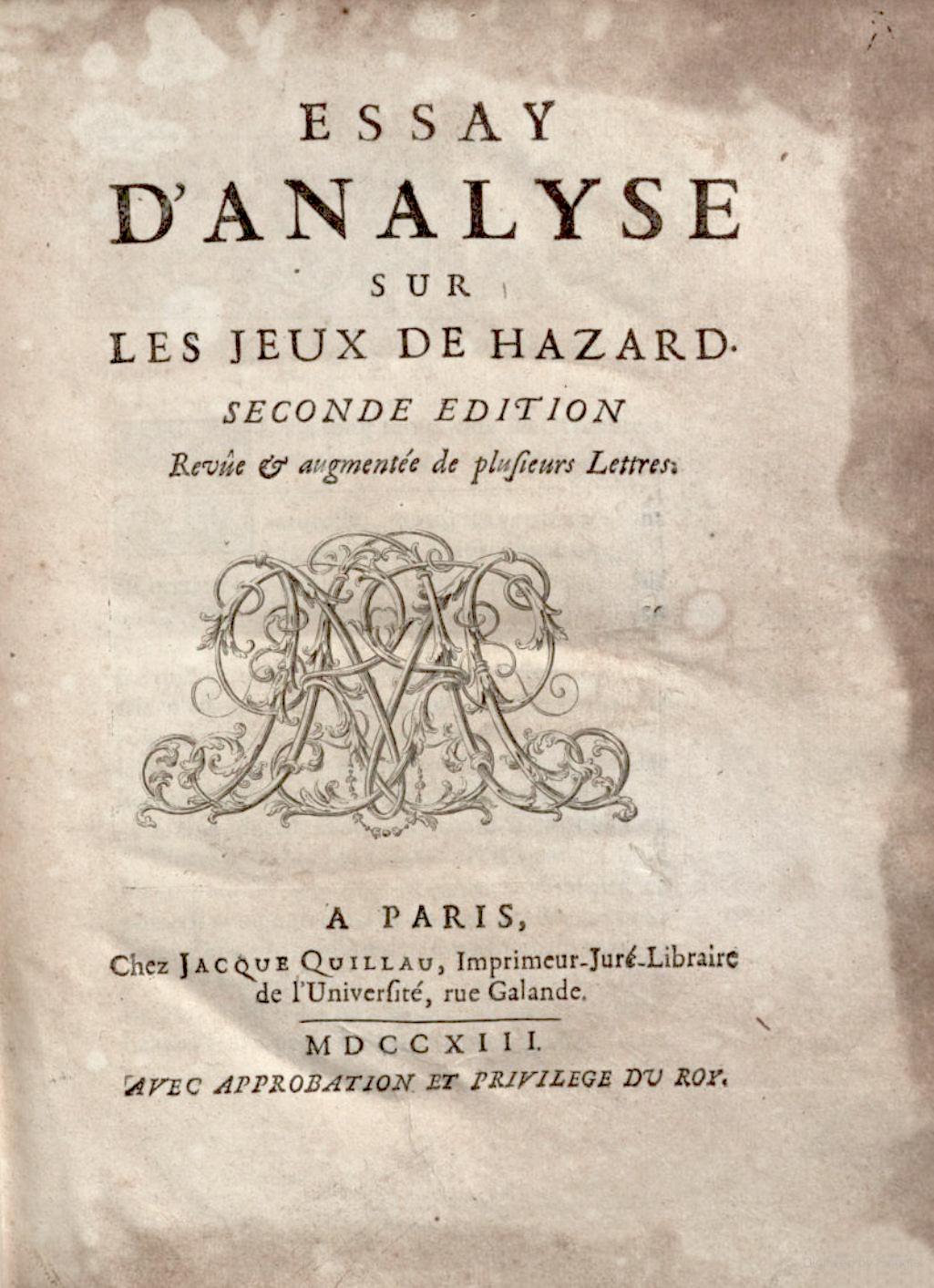
In the seventeenth and eighteenth centuries, academic activity was often carried out by letter. These letters were intended to be public documents that would be widely circulated and even published. The first versions of the St. Petersburg paradox appeared in a letter by Nicholas Bernoulli (the cousin of Daniel) to the French mathematician Pierre Remond de Montmort. The latter had published his Essay d'analyse sur les jeux de hazard (Analytic Essay on Games of Chance). In it, Montmort applied the theory of chance of the past century to many games of chance. The second edition of 1713 was greatly expanded and included a letter by Nicholas Bernoulli of September 9, 1713, that posed the first version of the paradox.
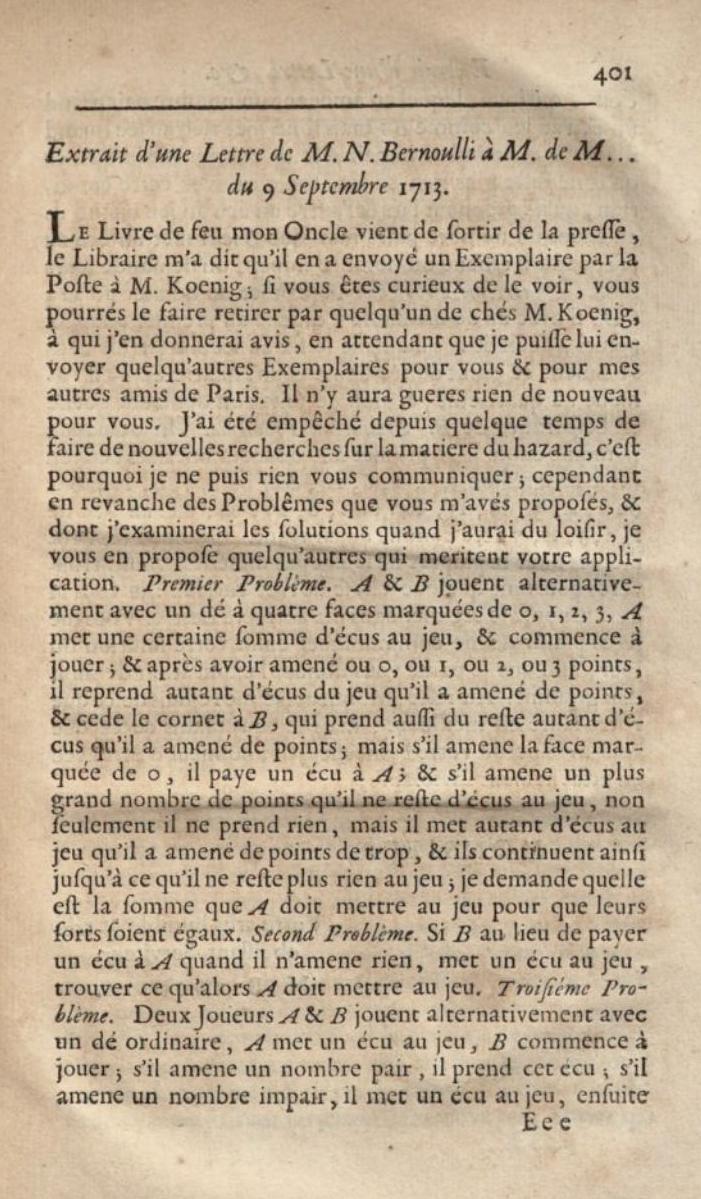
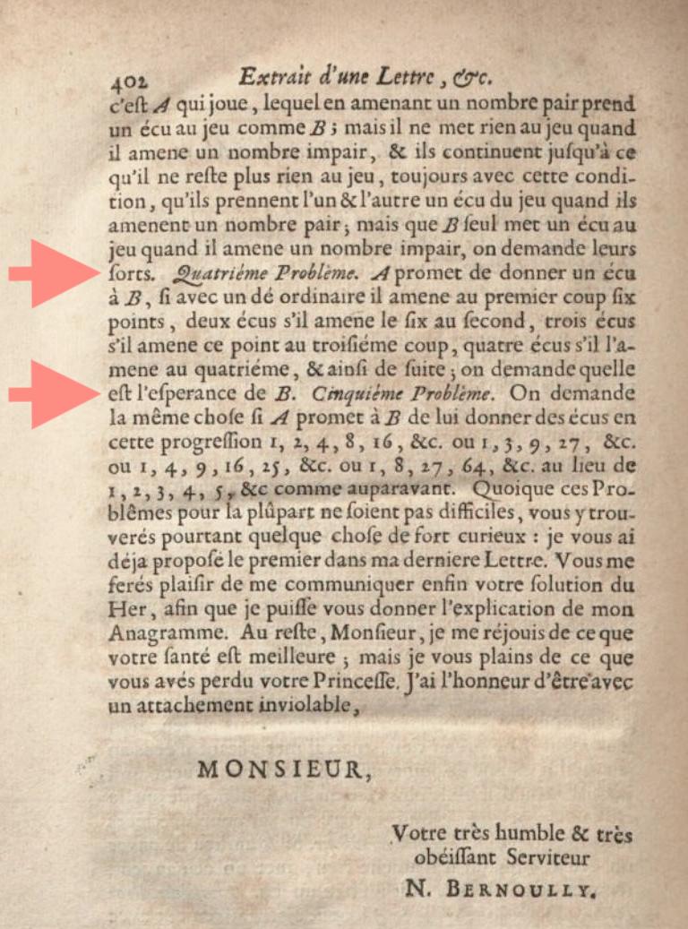
click images for larger version
The relevant part of N. Bernoulli's two page letter are the fourth and fifth problems posed by him (marked with the red arrows). In translation, the fourth problem reads:
Fourth Problem. A promises to give a coin to B, if with an ordinary die he brings forth 6 points on the first throw, two coins if he brings forth 6 on the second throw, 3 coins if he brings forth this point on the third throw, 4 coins if he brings forth it on the fourth and thus in order; one asks what is the expectation of B?
The fifth problem reads:
Fifth Problem. One asks the same thing if A promises to B to give him some coins in this progression 1, 2, 4, 8, 16 etc. or 1, 3, 9, 27 etc. or 1, 4, 9, 16, 25 etc. or 1, 8, 27, 64 instead of 1, 2, 3, 4, 5 etc. as beforehand. Although for the most part these problems are not difficult, you will find however something most curious.
N. Bernoulli just states the problems and expects Monmort to realize where the difficulty lies. If we examine them, we find that the fourth problem does not produce a troublesome infinite expectation. The rewards promised are paid the first time a six is cast with a regular die according to the schedule in the table:
Outcome  on toss number |
Probability | Reward in coins |
| 1 |
(1/6) | 1 |
2  |
(1/6)(5/6) | 2 |
| 3 |
(1/6)(5/6)2 | 3 |
| 4 |
(1/6)(5/6)3 | 4 |
| 5 |
(1/6)(5/6)4 | 5 |
| ... | ... | ... |
We would now calculate the expected reward by multiplying each probability with its reward and summing:
Expected reward
(1/6) + 2(1/6)(5/6) + 3(1/6)(5/6)2 + 4(1/6)(5/6)3 + 5(1/6)(5/6)4 + ... = 6
Thus far, N. Bernoulli's problems looks like familiar ones from the time. Infinite expectations arise, however, with N. Bernoulli's fifth problem. In the fourth problem, the rewards increase in an arithmetic progression, 1, 2, 3, 4, ... In the fifth problem, they increase geometrically. We can see the infinite expectation already with the first geometric progression, 1, 2, 4, 8, 16, ...
| Outcome on toss number |
Probability | Reward in coins | Probability x reward |
| 1 |
(1/6) | 1 | 0.16 |
| 2 |
(1/6)(5/6) | 2 | 0.28 |
| 3 |
(1/6)(5/6)2 | 4 | 0.46 |
| 4 |
(1/6)(5/6)3 | 8 | 0.77 |
| 5 |
(1/6)(5/6)4 | 16 | 1.28 |
| ... | ... | ... | ... |
The column added to the right shows that the terms to be summed in computing the expectation increase as we move down the table. A little arithmetic shows that the terms increase by a factor of 2x(5/6)=5/3 with each row. Since they increase in magnitude, the sum of these terms is infinite:
Expected value = ∞
Monmort, however, fails to see the difficulty. It is only in subsequent correspondence that N. Bernoulli explains the problem. He does this in a letter to Montmort of February 20, 1714. First he shows that the fourth problem presents no special challenges.
. . . It is true what you say that the last two of my Problems have no difficulty, nevertheless you would have done well to seek the solution, because it would have furnished you the occasion to make a very curious remark. Let the expectation of B be called x in the case of the 4th problem, you will have x = (1 + 5y)/6 (I name y the expectation of B when he is lacking the six on the first throw); now y is necessarily x + 1; because when he is lacking the six on the first throw, he expects to receive some coins in this progression 2, 3, 4, 5, 6, of which each term is one unit greater than the corresponding term of that here 1, 2, 3, 4. Substitute therefore x + 1 in place of y, and you will have x = (5x + 6)/6, and therefore x = 6. This which you would have found also by the route of infinite series.
Bernoulli uses an ingenious shortcut to arrive at the expectation of 6. It replaces summing the infinite series by a quicker computation. He writes the expectation as x, which is equal to the infinite series above:
x = (1/6) + 2(1/6)(5/6) + 3(1/6)(5/6)2 + 4(1/6)(5/6)3 + 5(1/6)(5/6)4 + ...
If we subtract 1/6 from both sides and multiply by (6/5) we recover:
(6/5)(x-1/6) = 2(1/6) + 3(1/6)(5/6)+ 4(1/6)(5/6)2 + 5(1/6)(5/6)3 + ...
The right hand side is just the original series, with the difference that the rewards are not 1, 2, 3, 4, ... but increased by one: 2, 3, 4, 5, ... That means that the right hand side is just the original expectation increased by 1. It must be x+1. Thus, the infinite sum reduces to:
(6/5)(x-1/6) = x+1
It is equivalent to N. Bernoulli's x=(5x+6)/6. A little algebra tells us that
x=6.
N. Bernoulli continues to explain that the fifth problem, the case of rewards in geometric progressions, leads to an infinite expectation. This, he notes, would oblige someone engaging in the game to pay an infinite entrance fee, or even more, and that would lead to a certain loss:
But if you follow the same analysis in the examples of the 5th problem as in the example of this progression 1, 2, 4, 8, etc, where you will have y = 2x, you will find x = (1 + 10x)/6 = −1/4, which is a contradiction. In order to respond to this contradiction, one might say that this fraction, regarded as having the negative denominator and consequently smaller than zero, is greater than 1/0, and that therefore the expectation of B is more than infinity, that which one finds also effectively by the method of infinite series. But it would follow thence that B must give to A an infinite sum and even more than infinity (if it is permitted to speak thus) in order that he be able to make the advantage to give him some coins in this progression 1, 2, 4, 8, 16 etc. Now it is certain that B by giving such a sum always would lose, since it is morally impossible that B not achieve six in a finite number of throws.
Instead of just computing the expectation directly as an infinite sum and showing that it is infinite, N. Bernoulli uses the same shortcut as he used on the fourth problem. For the series of rewards 1, 2, 4, 8, ..., the expectation is:
x = (1/6) + 2(1/6)(5/6) + 4(1/6)(5/6)2 + 8(1/6)(5/6)3 + 16(1/6)(5/6)4 + ...
If we subtract 1/6 from both sides and multiply by (6/5) we recover:
(6/5)(x-1/6) = 2(1/6) + 4(1/6)(5/6)+ 8(1/6)(5/6)2 + 16(1/6)(5/6)3 + ...
The right hand side is the same series for the expectation, with the exception that the rewards are not 1, 2, 4, ... but their doubles, 2, 4, 8, ... That is, the right hand side is double the original expectation, 2x.
The equation becomes
(6/5)(x-1/6) = 2x
A little algebra gives N. Bernoullli's solution:
x = -1/4
A negative answer is obviously incorrect. The infinite series sums terms all of which are positive. Bernoulli does not point out the obvious reason for this negative result. The trouble is that x is infinite, so that the equation (6/5)(x-1/6) = 2x is really just an indefinite
"∞ = ∞"
Trying to solve further for x to recover some finite value involves fallacious inferences.
To see a comparable fallacy, if y=∞, we can deduce from it the logically weaker condition y=2y-1. It is logicaly weaker since the equation y=2y-1 is compatible with two solutions: the original y=∞ and also y=1. This means that, when we solve the equation y=2y-1, we should arrive at two solutions, y=∞ and also y=1. We would need to take notice of other conditions involved in the posing of the problem to find which is the appropriate solution. Just inferring to y=1 as the solution would be a fallacy, if other conditions indicate that y=∞ is the appropriate solution.
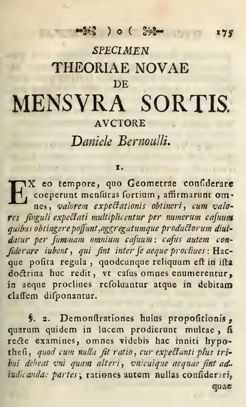
It was only 25 years after this correspondence that Daniel Bernoulli published his account of the paradox. The treatment became the best known presentation. Since it was published by the St. Petersburg Academy in St. Petersburg, Russia, the problem came to be know as the St. Petersburg problem or paradox.
click images for larger version
Daniel Bernoulli's purpose in discussing the paradox was to advocate for a particular solution, the diminishing utility of money, to which we now turn.
An early and still common response to the paradox was developed by the mathematician Gabriel Cramer and Nicholas' cousin Daniel Bernoulli. It notes that larger amounts of reward money cease to be as valuable to the player as smaller amounts. The first $1 of reward is prized. The next $1 after a $100 is surely still valued. But if the player were to be rewarded with $1,000,000, would an extra $1 still have the same value to the player as the first $1?
This diminution in value is tracked by "utility," which is the true value to the player of the amounts concerned. Here is a curve from D. Bernoulli's paper that displays the effect. The horizonal axis shows the numerical value of some amount in coins or ducats. The vertical axis show the corresponding utility. The flattening of the curve indicates that each extra unit is worth less in utility.
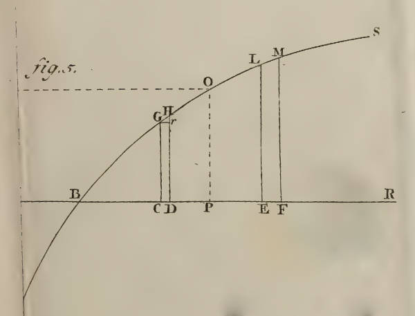
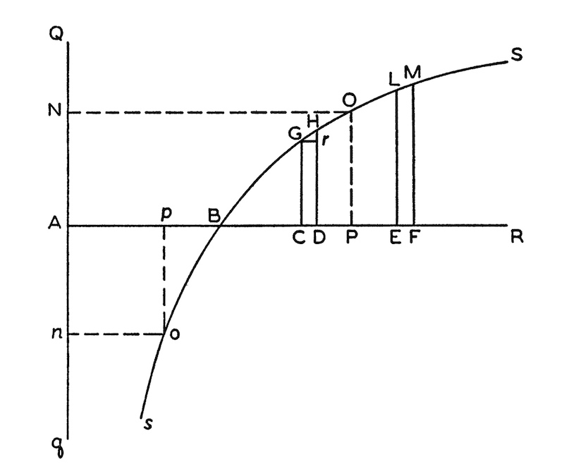
The original image on the left was truncated in the web source. The image on the right is the full figure from the translation.
The simplest version of the proposal was made by Cramer in correspondence of 1732 with Nicholas Bernoulli. (The correspondence was reproduced in Daniel Bernoulli's 1738 paper.) It is that that the utility--the true value of the rewards--increases only with the square root of the monetary amount. Hence 1 ducat has a utility √1 and is not reduced. But 100 ducats have a utility of √100 = 10.
In the simplest example considered by Cramer and D. Bernoulli, rewards in ducats were
1 with probability 1/2
2 with probability 1/4
4 with probability 1/8
8 with probability 1/16
...
The corresponding utilities are:
√1 = 1, √2 = 1.414, √4 = 2, √8 = 2.828, √16 = 4, ...
The expected utility is given by the infinite sum
√1/2
+ √2/4
+ √4/8
+ √8/16
+ ...
=
1 / (2 - √2)
The expected utility does not tell us how much the entrance fee should be for the game. Undoing the square root scaling recovers an amount in ducats, which is the fair entrance fee reported by Cramer:
1 / (2 - √2)2 = 2.9...
Below again I review historical details that readers may omit if they are eager to proceed with a more modern analysis.
D. Bernoulli's determination of utilities was more complicated. It factored in the player's fortune, represented by α. The larger this fortune, the less utility was accrued with each extra coin. The contribution to the total net utility of each reward in a game with many different rewards came though a term:
(α + reward)number of ways the reward comes about
All these terms are multiplied together and a root is extracted by raising the whole product to the power of (1/total number of ways rewards arise). The player's fortune, α, is subtracted for the final result.
For the example above, D. Bernoulli needs infinitely many equal chance ways that the rewards can arise. He represents this infinity by N and:
The probability 1/2 outcomes arise in N/2 cases.
The probability 1/4 outcomes arise in N/4 cases.
The probability 1/8 outcomes arise in N/8 cases.
The probability 1/16 outcomes arise in N/16 cases.
...
The net total utility of the game then becomes:
( (α + 1)N/2 (α + 2)N/4 (α + 4)N/8 ...)1/N - α
Needless to say, this formula is incoherent. If N represents infinity, then, then the entire expression is a mess. Raising to powers of N/2 etc. corresponds to raising to infinite powers and gives an infinite result. Raising to a power of 1/N corresponds to raising to the zeroth power. For finite numbers it returns unity. Raising an infinite number to the zeroth power gives no definite result. Overall, D. Bernoulli's formula corresponds to no well-defined result.
Nonetheless, D. Bernoulli can make all the terms in N cancel and produce a coherent result. It is a simple formal manipulation to raise each term in the infinite product to the power of 1/N and thereby eliminate the formal presence of N. It is a manipulation that would be correct if N were finite. For example:
( (α + 1)N/2 )1/N = (α + 1)1/2
The net total utility becomes
(α + 1)1/2 (α + 2)1/4 (α + 4)1/8 ... - α
which is a result independent of the dubious infinite N. The simplest case is of a player who starts with no fortune, α=0. Then the net total utility is just
11/2 21/4 41/8 81/16... = 2
In a sense, D. Bernoulli's analysis works. We would now carry out the same computation using a careful limit procedure and recover D. Bernoulli's final result.
There is, for me, an interesting historical footnote in this last computation. I have investigated how seventeenth century theories of chance did not use probability as their basic quantity. Instead they used a count of equally likely cases. Here D. Bernoulli is still using these older methods. They are inappropriate for the problem he addresses. It requites infinitely many equally likely cases. Using them to compare outcomes, each corresponding to infinitely many cases, is dangerous and can easily lead to fallacies. To proceed by case counting is standard enough that he struggles on with it and can still arrive at a serviceable result.
While a resolution based on the diminishing utility of money is often reported, it is quite unsatisfactory. It seeks to escape the difficulty by changing the problem posed. It tells us how someone who has this diminished utility in money might find the problem. But that was not the original problem. We considered someone who values money according to the dollar amount. The escape, in any case, might sometimes easily be evaded simply by increasing the profile of the rewards offered such that the expected reward in utility terms is still infinite.
This is also N. Bernoulli's assessment of this attempt at a solution to the problem. He gave just this criticism to his cousin Daniel in a letter of April 5, 1732:
. . . I thank you for the effort that you yourself have given to me communicating a copy of your Specimen theoriae novae metiendi sortem pecuniariam; I have read it with pleasure, and I have found your theory most ingenious, but permit me to say to you that it does not solve the knot of the problem in question. The concern is not to measure the use or the pleasure that one derives from a sum that one wins, nor the lack of use or the sorrow that one has by the loss of a sum; the concern is no longer to seek an equivalent between the things there; but the concern is to find how much a player is obliged according to justice or according to equity to give to another for the advantage that therein accords him in the game of chance in question, or in other games in general, so that the game is able to be deemed fair, as for example a game is considered fair, when the two players bet an equal sum on a game under equal conditions,...
In his earlier letter to Montmort of February 20, 1714, N. Bernoulli had already given his own solution to the problem. It was:
From all this I conclude that the just value of a certain expectation is not always the average that one finds by dividing by the sum of all the possible cases the sum of the products of each expectation by the number of the case which gives it; that which is against our fundamental rule. The reason for this is that the cases which have a very small probability must be neglected and counted for nulls, although they can give a very great expectation. For this reason one is able yet to doubt if the value of the expectation of B in the case of the 4th problem such as I have found above, is not too great. Similarly in Lotteries where there are one or two quite great Lots, the just value of a single ticket is smaller than the sum of all the money of the Lottery divided by the sum of all the tickets, supposing that the number of those here is also very great. This is a remark which merits to be well examined.
This escape seems to me to be the right one. The huge payoffs that lead to the infinite expectation occur with very small probability. Any reasonable assessment of a fair entrance fee ought to proceed with the recognition that these very small probability events are so unlikely that they should be ignored. A reward of $1024 will happen with probability 1/210 = 1/1024. A reward of $1,048,576 will happen with probability 1/220 = 1/1048576.
The difficulty is to determine just which of these low probability outcomes should be ignored. The answer--provided by William Feller below--is that the number of times the game is played will determine which are to be ignored.
If we play just once, we are very unlikely to encounter the outcome with probability 1/210 = 1/1024. That is the case of nine tails is a row, followed by a head:
If, however we were to play the game 1,024 times, then we would expect this outcome appear roughly once in our game play. That means that the fair entrance fee ought to change with the number of games we commit to play. If we commit to play just one game, then the fee should be quite small. We are very unlikely to recover the $1,024 reward. If, however, we were to pkay 1,024 times, then we might well secure the $1,024 reward. A fair entrance fee would have to be larger to reflect that possibility.
Just how a fair entrance fee must vary with the number games played will be determined below, following Feller's analysis. But first, we must ask why the infinite expected value of the game no longer controls the size of a fair entrance fee.
The strongest justification, in my view, for using expected values to govern our decisions is that expected values are well approximated by the average returns secured over many repetitions of the same decision problem. In game play, if we choose the option with some given expected value, our average gain will approach that expected value in long run of many plays.
The key idea in the justification is the notion of a game played in the "long term," as opposed to the "short term." By "long term," I mean that there are sufficiently many repetitions of the game that the weak law of large numbers can be brought to bear. Games played for fewer repetitions are being played in the short term.
The weak law of large numbers has been discussed in the Probability Theory Refresher. In brief, it assures us that, in many repeated plays, the frequencies of the various outcomes will approach their probabilities. More precisely it says that we can pick any degree of closeness between the frequencies and the probabilities. Then, by repeating the game often enough, we can be sure with arbitrarily high probability that the frequencies lie within that degree of closeness to the probability.
This approach of the frequencies to the probabilities is then imprinted on the expectations. As the frequencies approach the probabilities, the rewards paid by the repeated runs of the game, when averaged over the runs, approaches the expected rewards.
In my view (as explained earlier), expected value is only a useful guide in the longer term case. For it is useful only in so far as it tells us what to expect of the averages in many plays. In the short term, it gives us little.

A familiar example of a short term game is a lottery. The expected return on any lottery ticket is negative. Otherwise, a lottery cannot cover its operating costs, let alone run at a profit. However, when someone buying a $1 ticket is told that the expected return is $0.5, that is unlikely to dissuade them. A lottery ticket purchase is a game played in the short term. The attraction is the possibility of a big win now, not whether the purchase of lottery tickets will be profitable on average in the long run.

The lottery game can become a long term game when the player participates in so many lotteries that there are many losing tickets and some winning ones. More realistically, we might have a well-funded cartel that purchases many tickets over a long period in many lotteries.
For such a cartel, they key concern is whether their expected returns will exceed the cost of the tickets over the long term life of their purchases. That is, the decision of whether to engage in the lotteries will be determined by the expected returns in comparison with the entrance costs.
For most games, such as lotteries, the short term can be converted into the long term merely by playing the game often enough. In the short term, there is little security in the outcome. A player might lose; or a player might gain a lot. If, however, the game is played repeatedly, eventually the losses and gains on average smooth out the peaks and valleys of wins and losses. The averages approach the expected values and the expectations become good guides to the net, long term rewards.

https://commons.wikimedia.org/wiki/File:Car_pictogram.svg
Another more practical example of a short term game is the practice of buying insurance, on, for example, a car. We buy the insurance even though we know that the expected return in the unlikely event of a claim will be less than cost of the policy. It must be so. Otherwise the insurance company could not stay in business. Insuring a single car is like a single play in the insurance game.

If, however, we operated a fleet of many cars, our thinking would change. Insuring the whole fleet is like playing the insurance game many times. We are now operating in the long term. We expect a small number of claims among the cars of our fleet. In deciding whether to buy insurance on each car, we would consider the cost to us of those losses averaged over the whole fleet. Since the insurance company must cover its costs and even make a profit, the total cost to purchase insurance would exceed the total losses that the insurance would make good. In average terms, the loss averaged over each car would be greater than the negative expected return on a policy bought on each car. We would use the expected return to guide our decision not to insure the cars. It is advantageous to "self-insure," that is, to cover any losses out of our existing funds.
The distinctive feature of long term play is that, on repeated plays, the average net returns eventually stabilize to some constant value that matches the probabilistically expected value. What William Feller recognized is that the St. Petersburg game is an exception to this generic behavior. It does not matter how many times a player plays. The play always has a short term character. The gains never settle down to some stable average. Instead, as the player plays repeated games, the average rewards keep increasing. They are moving towards the infinite expected reward of $∞. They are on the way to stabilization to the average. However they never attain it. The average reward is always finite and thus always infinitely far away from the infinite expectation, no matter how many times the game is played.
The more games that are played, the more likely is it that a high reward-low probability outcome is realized. With still more games played, it is still more likely that the player secures a still larger reward. It follows that there can be no single entrance fee that makes the game fair. For the rewards a player expects depend essentially on how many games the player is willing to play. In Feller's resolution of the paradox, the player is asked to state in advance how many games the player will play. A fair entrance ticket is then computed according to the number of games declared.
The value of that fair entrance ticket increases with the number of games that will be played. When that number becomes very large, Feller found a simple relation between the number of games to be played and the fair entrance ticket. It is:
If a player will play a large number of games, 2n, then the fair entrance fee per game is approximately n.
The approximation is poorer for smaller values of n, but improves as n becomes larger. It is tolerably good when n is as large as 100. In that case, the player undertakes to play 2100 games.The fair entrance fee for each game is $100. That means that the total entrance ticket payment by the player is $100 x 2100. That is a large entrance ticket. What justifies it is that the player will be returned that amount with high probability over the course of play. It is a fair entrance fee since neither the player nor someone offering the game will come out ahead on average.
Once the player has secured the agreement on the $100 entrance fee, it is in the best interests of the player to insist that all 2100 games be offered. If they are not offered and the player cannot play all of them, then the entrance fees the player paid for the smaller number of games exceed the fair entrance fee.
As a preliminary to Feller's analysis, it is
convenient to define a truncated St. Petersburg game. In it, there is a maximum
number of times that the coin will be tossed. Call it "n." If no
head has appeared in these n tosses, then the game is over and the player
receives no reward.
| Toss on which head first appears | 1 | 2 | 3 | ... | n |
| Reward | $2 | $4 | $8 | ... | $2n |
| Probability | 1/2 | 1/4 = 1/22 | 1/8 = 1/23 | ... | 1/2n |
| Expected reward contribution | $2x1/2 = $1 | $4x1/4 = $1 | $8x1/8 = $1 | ... | $2nx1/2n=$1 |
| Expected reward, $n = | $1 + |
$1 + |
$1 + |
... |
+ $1 |
This truncated game behaves like familiar games. A short term player who will play the game only once may not be too concerned with the expected reward. The excitement of a possible win of a large reward of $2n may be enticement enough to play the game.
If the game is played many times, however, the expected reward of $n becomes more significant. The law of large numbers will start to become relevant. For this to happen, the player would need to play many times. The largest reward is 2n. It occurs with the least of all the probabilities, 1/2n. On average we expect it to arise once in 2n games. That gives us a very rough estimate of how many times the game must be played for long term considerations to apply.
If a player plays 2n times, the player would receive, in very rough estimate, rewards of:
$2 in 1/2 the games = 2n/2
games = 2n-1 games
$4 in 1/4 the games = 2n/4 games = 2n-2 games
...
$2n in 1/2n the games = 2n/2ngames
= 1 game
Summing, the total reward is
$2 x 2n-1 + $4 x 2n-2 + ... + $2nx1 = nx$2n
Since we are assuming 2n plays, this total reward would average out to a reward of $n for each game. That is, the expected reward would match, near enough, the average reward actually received in many games.
This last result conforms with the law of large numbers. A decision to play would then be based on a comparison of the entrance fee with the expected reward on each game. If they match, the game would be judged fair. A smaller entrance fee would then be judged favorable to the player. A larger entrance fee would be unfavorable to the player.
The core idea behind Feller's analysis is that the entrance fee a player is to be charged for the St. Petersburg game must increase with the number of games the player will play.
Informally we can see why this might be reasonable. A player who plays just once is likely only to win a smaller reward. With great probability, the reward will come after only a few tosses. If, however, the player plays many times, then the chance of a highly profitable long run of tails increases. Because of the structure of the game, a player who does this can gain a significant advantage over the player who plays just once, even in the averages.
To get a sense of how this works, imagine a player who plays 2n games. On average, this player expects to win roughly on the same schedule we saw for the truncated game:
$2 in 1/2 the games = 2n/2
games = 2n-1 games
$4 in 1/4 the games = 2n/4 games = 2n-2 games
...
$2n in 1/2n the games = 2n/2n
games = 1 game
Loosely speaking, the game looks to the player to be just like a play of 2n games of the truncated St. Petersburg game, where the coin tosses are truncated to n tosses only.
This schedule then leads to the same average reward:
$n on average per game among the 2n games played.
This result sets what is a fair entrance fee. If a player enlists to play 2n games, then a fair entrance fee is $n per game or $nx2n for all 2n games. If the entrance fee is less, the game favors the player who will on average make a net gain. If the entrance fee is greater than $n, then the game is unfavorable to the player, who will on average make a net loss.
Hence the fair entrance fee for the player increases without limit as the number of games to be played increases. This is the perpetual short term behavior of the St. Petersburg game. No matter how many times the game is played, the rewards it returns do not settle down to stable values, as is the familiar behavior of common games. Rather, the average reward per game keeps increasing indefinitely; and they do so in direct proportion with the number of games played, n.
The above argument is quite imprecise. It is intended only to give a loose sense of what leads to the size of the fair entrance fee proposed by Feller.
Feller gives a precise derivation of a result that justifies this fair entrance fee in the place cited above. He shows that when the number of games played 2n is large, then, with high probability, the average reward the player will accrue per game is close to $n. In a result that mimics the law of large numbers, Feller shows that the closeness of the average reward to $n can be made arbitrarily small and with arbitrarily great probability merely by playing a sufficiently large number n of games.
(What follows are some technical details that may be skipped unless they seem interesting.)
We can tighten the above analysis to bring it closer to Feller's in the following way. The determination of the average reward of $n per game tacitly makes an important assumption. It is that all the first heads in all the 2n games occur within the first n tosses. That is, the assumption is that these first 2n games proceed almost exactly like the truncated game. That is an unrealistic assumption.
A short calculation shows why it is unrealistic. The probability that all heads come within the first n tosses in all the games can be computed fairly easily:
Probability that heads comes first after n tosses in one game = 1/2n.
Probability that heads comes first within the first n tosses in one game = (1-1/2n).
Probability that heads comes first within the first
n tosses in 2n games
= (1-1/2n) x (1-1/2n) x ...(2n
times) ... x (1-1/2n)
= (1-1/2n)2n ≈
1/e = 0.3678....
This shows that the simplifying assumption of the earlier analysis holds only with probability 0.3678...., that is, roughly 1/3rd of the time. Since this value of 1/e is independent of n, this difficulty will persist no matter how many games are played.
It follows that mostly, that is with probability of roughly 0.63, some of the games in a set of size 2n will have the first heads outcome after n tosses. This turns out not be a major problem for the estimate of average rewards. For with high probability, those later heads outcomes will arise in the first few tosses subsequent to the n tosses. They will have a slight effect on the average payout. However as n becomes large, the effect will be negligible.
To see this effect more precisely, consider the probability that all the first heads outcomes arise not in the first n tosses, but in the first n+1 tosses. Following the model above, the probability of this occurrence is
(1-1/2n+1) x (1-1/2n+1) x ...(2n
times) ... x (1-1/2n+1)
= (1-1/2n+1)2n = (1-1/2n+1)2(n+1).(1/2)
≈
(1/e)1/2 = 0.6065....
If this case is realized, the average reward is n+1.
This computation can be continued for more coin tosses. The probability that all first heads arise in the first n+2 coin tosses is computed analogously as
(1-1/2n+2) x (1-1/2n+2) x ...(2n
times) ... x (1-1/2n+2)
= (1-1/2n+2)2n = (1-1/2n+1)2(n+2).(1/4)
≈
(1/e)1/4 = 0.7788....
If this case is realized, the average reward is n+2.
Proceeding this way, we arrive at the results in the table below:
| Number of tosses that contain all first heads | Probability | average reward |
| n | ≈ 1/e = 0.3678... | n |
| n+1 | ≈ (1/e)1/2 = 0.6065... | n+1 |
| n+2 | ≈ (1/e)1/4 = 0.7788... | n+2 |
| n+3 | ≈ (1/e)1/8 = 0.8824... | n+3 |
| n+4 | ≈ (1/e)1/16 = 0.9394... | n+4 |
| n+5 | ≈ (1/e)1/32 = 0.9692... | n+5 |
To summarize: the simplified analysis of the last section tells us that, with high probability, the average reward when 2n games are played is $n. This then justifies Feller's value of a fair entrance ticket of $n. The difficulty with the simplified analysis is that it requires the case to be one in which all the first heads arise in the first n tosses. We see in the table above that this condition is less probable.
While we cannot assume that the first heads always arise in the first n tosses, the table above shows us that we can assume something close enough to it for our purposes. This is, with increasing probability, we can assume that all the first heads come within the first n tosses or a few after them. If we extend our reach to the first n+5 tosses, the table shows, there is a probability of 0.97 that that we have encompassed all the heads. Then the average reward per game increases just to n+5.
Feller's result concerns what happens in the limit of very large n. If we consider large n, say n=100, n=1000, n=10,000, then the difference between n and n+5 becomes negligible in ratio when n is large. Thus for large n, Feller's $n entrance fee matches the average rewards expected with high probability.
As you may have already noticed, the number of games under discussion is very large. If we choose n=100, then the number of games to be played is
2100≈ 1.27 x 1030 ≈ 1,270,000,000,000,000,000,000,000,000,000
In practical terms, we should not expect anyone to play this many games! We would, however, need to commit to this many games if we are to use Feller's result of $100 as a reasonable estimate of the fair entrance ticket. (A better estimate using probability 0.97 in the above table is $105, which is 5% larger.)
If our concern is simply to discover if there is a method of determining a fair entrance ticket, the need for this large number of games may not be troublesome. If we are looking for practical advice on how to play the game, then Feller's result is unhelpful. We do get helpful results, however, from a small modification to Feller's analysis. The results needed are in the table above.
A more realistic strategy for playing the St. Petersburg game would be for a player to commit to playing a small number of games, such as 25 = 32 games. We then read off from the table, that, with probability 0.97, all the heads in all the games will occur in the first n + 5 = 5 + 5 = 10 games. The average reward per game is also n + 5 = 5 + 5 = $10.
Commit to play 32 games with entrance fee $10 per game
While these matters should be resolved by well-founded calculations, it is plausible that this entrance ticket is fair. With probability 0.97, all the heads will occur in the first 10 tosses. These are the tosses indicated in the table below. The associated rewards and their probabilities are also shown.
| Toss on which heads first appears | 1 | 2 | 3 | 4 | 5 | 6 | 7 | 8 | 9 | 10 |
| Reward | $2 | $4 | $8 | $16 | $32 | $64 | $128 | $256 | $512 | $1024 |
| Probability | 1/2 | 1/4 | 1/8 | 1/16 | 1/32 | 1/64 | 1/128 | 1/256 | 1/512 | 1/1024 |
Considering the synopsis of likely play displayed in this table, an entrance ticket of $10 seem much more reasonable than the infinite entrance fee or arbitrarily large entrance fee indicated by the original expected reward calculation.
In the exchange paradox, an amount of money is placed in one envelope and twice that amount in a second envelope.

head siluouette from
https://commons.wikimedia.org/wiki/File:Head_silhouette.svg
The two envelopes are shuffled thoroughly. Player 1 is given one of them and a second player is given the other envelope. The players will keep the money in their envelopes.

Both players are now given the opportunity to swap their envelopes with that of the other player. Player 1 reasons as follows:
"My envelope has some amount in it: "x," say.
The other envelope has either half that amount, x/2, or twice that amount,
2x. If I swap with the other player, I may get either. the probability of
each case is equal to 1/2. Hence my expected gain in swapping is:
Expected amount in other envelope
minus actual
amount in my envelope now
= (1/2) . 2x + (1/2) . (x/2) - x
= (5/4) . x - x
= x/4
That is, if I swap, I have an expected gain of x/4.
Therefore I should swap."
Thus far, the decision problem seems straightforward. The problem, however, is that the game satisfies two conditions:
• (symmetry) The game is perfectly symmetric. Both players can reason identically and come to the conclusion that both players profit from swapping.
• (zero sum) Any gain one player makes is at the cost of the other player and vice versa. Hence both cannot profit from swapping.
We have a true contradiction:
"Symmetry" and the expected gain computation lead to the conclusion: both players gain if they swap.
"Zero sum" leads to the negation of this conclusion conclusion: It is not the case that both players gain if they swap.
This exchange paradox is set up remarkably easily. This ease is deceptive. It has produced an extended literature with a range of reactions and solutions proposed. I will not try to survey them here. Rather I will pursue what I think is the core difficulty. Its identification resolves the contradiction.
The paradox derives from the failure of the expected gain to be a well-defined quantity. Here the difficulties go one step beyond what we saw in the St. Petersburg paradox. There the expected value criterion failed since the expected value took on an infinite value. In that case, at least, the expected value had a definite, if awkward, value. In the exchange paradox, the problem is worse. The expectation has no well-defined value at all.
If we remove the expected value computation from the paradox, we no longer have both players expecting to gain in a swap. Without that, both conditions of symmetry and zero sum can be maintained. They merely now entail that neither player gains in swapping.
The example of the infinite checkerboard illustrates how the expected gain in the exchange paradox can have no well-defined value.
Consider an infinite checkerboard. The amounts +1 and -1 are placed on alternating squares as shown.
| +1 | -1 | +1 | -1 | +1 | -1 | +1 | -1 | ... |
| -1 | +1 | -1 | +1 | -1 | +1 | -1 | +1 | ... |
| +1 | -1 | +1 | -1 | +1 | -1 | +1 | -1 | ... |
| -1 | +1 | -1 | +1 | -1 | +1 | -1 | +1 | ... |
| +1 | -1 | +1 | -1 | +1 | -1 | +1 | -1 | ... |
| -1 | +1 | -1 | +1 | -1 | +1 | -1 | +1 | ... |
| +1 | -1 | +1 | -1 | +1 | -1 | +1 | -1 | ... |
| -1 | +1 | -1 | +1 | -1 | +1 | -1 | +1 | ... |
| ... | ... | ... | ... | ... | ... | ... | ... | ... |
What is the total amount, net, on the checkerboard? One might think that an answer is given simply by adding up all the amounts in the squares. The difficulty is that there are different ways of adding the amounts and these different ways give different results, or no result at all.
For example, we can add up the amounts by pairs. we first sum adjacent amounts in the blue squares and in the green squares, as shown. Then we sum all those sums.
| +1 | -1 | +1 | -1 | +1 | -1 | +1 | -1 | ... |
| -1 | +1 | -1 | +1 | -1 | +1 | -1 | +1 | ... |
| +1 | -1 | +1 | -1 | +1 | -1 | +1 | -1 | ... |
| -1 | +1 | -1 | +1 | -1 | +1 | -1 | +1 | ... |
| +1 | -1 | +1 | -1 | +1 | -1 | +1 | -1 | ... |
| -1 | +1 | -1 | +1 | -1 | +1 | -1 | +1 | ... |
| +1 | -1 | +1 | -1 | +1 | -1 | +1 | -1 | ... |
| -1 | +1 | -1 | +1 | -1 | +1 | -1 | +1 | ... |
| ... | ... | ... | ... | ... | ... | ... | ... | ... |
Then the total amount is
(1 - 1) + (1 - 1) + (1 - 1) +
= 0 + 0 + 0 + ... =0
We might also add them by the paired diagonals shown:
| sum on diagonal | |||||||||
| +1 | +1 | -1 | +1 | -1 | +1 | -1 | +1 | +1 | ... |
| +1 = -2+3 | -1 | +1 | -1 | +1 | -1 | +1 | +1 | +1 | ... |
| +1 | -1 | +1 | -1 | +1 | +1 | +1 | -1 | ... | |
| +1 = -4+5 | -1 | +1 | -1 | +1 | +1 | +1 | -1 | +1 | ... |
| +1 | -1 | +1 | -1 | +1 | -1 | +1 | +1 | ... | |
| +1 = -6+7 | -1 | +1 | -1 | +1 | -1 | +1 | +1 | +1 | ... |
| +1 | -1 | +1 | -1 | +1 | +1 | +1 | -1 | ... | |
| ... |
-1 | +1 | -1 | +1 | +1 | +1 | -1 | +1 | ... |
| ... | ... | ... | ... | ... | ... | ... | ... | ... |
Then the total amount is
1 + (-2 + 3) + (-4 + 5) + (-6 + 7) + ...
= 1 + 1 + 1 + 1 + 1 + ... = ∞
Here is a closely related addition by a different pairing of the diagonals:
| sum on diagonal | |||||||||
| -1 = +1-2 | +1 | -1 | +1 | -1 | +1 | -1 | +1 | 1 | ... |
| 1 | +1 | -1 | +1 | -1 | +1 | -1 | +1 | ... | |
| -1 = +3-4 | +1 | -1 | +1 | -1 | +1 | -1 | +1 | 1 | ... |
| 1 | +1 | -1 | +1 | -1 | +1 | -1 | +1 | ... | |
| -1 = +5-6 | +1 | -1 | +1 | -1 | +1 | -1 | +1 | 1 | ... |
| 1 | +1 | -1 | +1 | -1 | +1 | -1 | +1 | ... | |
| -1 = +7-8 | +1 | -1 | +1 | -1 | +1 | -1 | +1 | 1 | ... |
| 1 | +1 | -1 | +1 | -1 | +1 | -1 | +1 | ... | |
| ... | ... | ... | ... | ... | ... | ... | ... | ... | ... |
We now have a quite different result:
(1 - 2) + (3 - 4) + (5 - 6) + ...
= - 1 - 1 - 1 - 1 - ... = -∞
These summations so far give definite results, even if different. Another summation gives no definite result. Again we sum along the diagonals:
| sum on diagonal |
|||||||||
| +1 |
+1 | -1 | +1 | -1 | +1 | -1 | +1 | -1 | ... |
| -2 |
-1 | +1 | -1 | +1 | -1 | +1 | -1 | +1 | ... |
| +3 |
+1 | -1 | +1 | -1 | +1 | -1 | +1 | -1 | ... |
| -4 |
-1 | +1 | -1 | +1 | -1 | +1 | -1 | +1 | ... |
| +5 |
+1 | -1 | +1 | -1 | +1 | -1 | +1 | -1 | ... |
| -6 |
-1 | +1 | -1 | +1 | -1 | +1 | -1 | +1 | ... |
| +7 |
+1 | -1 | +1 | -1 | +1 | -1 | +1 | -1 | ... |
| -8 |
-1 | +1 | -1 | +1 | -1 | +1 | -1 | +1 | ... |
| ... |
... | ... | ... | ... | ... | ... | ... | ... | ... |
The summation is:
1 - 2 + 3 - 4 + 5 - 6 + ...
This summation converges to no definite result. Rather the partial sums alternate between +1 and -1 indefinitely:
1
= 1
1 - 2 = -1
1 - 2 + 3 = 1
1 - 2 + 3 - 4 = -1
1 - 2 + 3 - 4 + 5 = 1
1 - 2 + 3 - 4 + 5 - 6 = -1
...
In short, there is no definite amount that represents the summation of all the amounts on the checkerboard.
However there is a trap lurking in the example. If we were to implement only one of the summation schemes indicated above, we might erroneously come to the conclusion that the summation has a definite value. For example, the first summation by individual pairs seems natural since we know that there are as many +1 and -1. So we might favor the first summation to zero. That would be a mistaken conclusion since it neglects all the other summation schemes. That one summation seems natural is no basis for dismissing the rest.
The trap just sketched for the checkerboard problem is the same trap that leads to a paradox in the exchange problem.
To see it, we need to specify the problem more precisely. The easy analysis just assumes that the first player's envelope has "x" in it. A computation is carried out over x and then a dangerous assumption is made: whatever we find for some specific x, say $16, will be true for a probabilistic aggregation of all possible values of x. This dangerous assumption is false.
For a specific value of x, the expected gain on swapping is well defined. It is
(1/2) x $32 + (1/2) x $8 - $16 = $4
We shall see that, if we allow x to have a sufficient range of values to meet the conditions of the problem, then the expectation ceases to be well-defined.
It is essential for the problem that the range of values that x can take is infinite. For otherwise, there will be a greatest value for x. That would appear as a special case in the computation of expectations. If a player has this maximum value, then expectation of a gain on x/4 for all x on swapping. If the player has the maximum value, then swapping leads to an assured loss. (This loss then cancels out any expected gains arising from smaller values of x.)
The specification of the problem does not indicate just what range of amounts may be in the envelopes. A set that is sufficient to meet the conditions of the problem is:
Possible amounts in each envelope: $1, $2, $4, $8, $16, ...
With these possible amounts, the outcome space consists of all adjacent pairs of amounts:
player 1 has $1, player 2 has $2
player 1 has $2, player 2 has $1
player 1 has $2, player 2 has $4
player 1 has $4, player 2 has $2
player 1 has $4, player 2 has $8
player 1 has $8, player 2 has $4
and so on indefinitely.
All of these pairs are equally probable.
We can represent these pair comprising the outcome space as columns in a table.
| Player 1 | 1 | 2 | 2 | 4 | 4 | 8 | 8 | 16 | 16 | 32 | ... |
| Player 2 | 2 | 1 | 4 | 2 | 8 | 4 | 16 | 8 | 32 | 16 | ... |
We can now compute what each player would gain,
were the player to swap:
| Player 1 | 1 | 2 | 2 | 4 | 4 | 8 | 8 | 16 | 16 | 32 | ... |
| Player 2 | 2 | 1 | 4 | 2 | 8 | 4 | 16 | 8 | 32 | 16 | ... |
| Player 1 gains in a swap | +1 | -1 | +2 | -2 | +4 | -4 | +8 | -8 | +16 | -16 | ... |
| Player 2 gains in a swap | -1 | +1 | -2 | +2 | -4 | +4 | -8 | +8 | -16 | +16 | ... |
Consider the expected gain that player 1 would make if player 1 swaps. The gains corresponding to each outcome are in the third row: +1, -1, +2, -2, +4, -4, ... Each of these has the same probability since each pair in the outcome space has equal probability. If that probability is some small amount ε:
Expected gain to player 1 in a swap
= ε ( 1 - 1 + 2 - 2 + 4 - 4 + 8 - 8 + 16 - 16 + ... )
Digression: A serious complication in this computation is that the probability distribution for this outcome space cannot be normalized to unity. That is, we have a countable infinity of outcomes each with probability ε. If we set ε>0, then summing an infinity of them leads to an infinite total probability for the whole outcome space. It violates the normalization axiom that the probability of the total outcome space is one. If we set ε=0, then the summation gives a total probability of zero, which again violates the normalization axiom.
A careful but tedious solution to the problem is to replace the assumption of equal probability of each outcome by an assumption of diminishing probability as the amounts in the pairs become large, such that all the probabilities sum to one.
This tedious solution works, but makes the computations messy without adding any illumination. While is it strictly impermissible, we can proceed with the above formula if we assume that the probability ε is greater than zero, but infinitesimally small, so that normalization of the probability measure is not compromised. This liberty does not affect the basic ideas of the analysis and I will proceed with it.
The infinite summation fails to have a well-defined value in the same way that the summation in the checkerboard problem fails to have a definite value. That is, we can compute the sum in different ways and get different results.
The simplest summation ends up concluding that no player has an advantage. That is we group the terms such that they pair-wise cancel to zero:
Expected gain to player 1 in a swap
= ε ( (1 - 1) + (2 - 2) + (4 - 4) + (8 - 8) + (16 - 16) + ... )
= ε ( 0 + 0 + 0 + 0 + 0 + ...) = 0
The analysis attributed to player 1 above, however, groups the terms differently. That analysis considered what happens if the player has an amount x. The two possible outcomes are then that the other player has x/2 and 2x. for example, in case player 1 has x=$2, then the other player may have $1 or $4. Applying this to all possible values of x, player 1 groups the terms in the summation as:
Expected gain to player 1 in a swap
= ε ( 1 + (- 1 + 2) + (- 2 + 4) + (- 4 + 8) + (- 8 + 16) + ... )
= ε ( 1 + 1 + 2 + 4 + 8 + ...) = ε x ∞ > 0
With this summation, player 1 concludes that there
is a positive expected gain in swapping so
that it is desirable.
Player 2 can carry out the same calculation on the fourth row of the table, which records player 2's gains. It will correspond to a different summation of the expected gain of player 1. The order of the gains in the table makes it easy to represent player 1's groupings, but less clear for player 2's. Player 2's grouping in the summation correspond to the boldface pairs:
( 1 - 1 + 2 - 2
+ 4 - 4 + 8 - 8 + 16 - 16 + ... )
( 1 - 1 + 2 - 2 + 4 - 4 + 8 - 8 + 16 -
16 + ... )
( 1 - 1 + 2 - 2 + 4 - 4 + 8 - 8 + 16 -
16 + ... )
( 1 - 1 + 2 - 2 + 4 - 4 + 8 - 8 + 16 - 16
+ ... )
...
Grouping these terms together, player 2's summation of player 1's expectation sums to:
Expected gain to player 1 in a swap
= ε ( -1 + (1 - 2) + (2 - 4) + (4 - 8) + (8 - 16) + ... )
= ε ( -1 - 1 - 2 - 4 - 8 - ...) = ε x -∞ < 0
Thus player 2 computes the expected gain for player
1, if they swap, to be negative, which means that there is a positive
expected gain for player 2.
These three ways of carrying out the summation are just three of infinitely many ways that it could be summed. These different ways can produce any result at all or, as with the case of the checkerboard, no definite result. We conclude that the expected value of a swap can provide no guide to the players since the quantity is not well-defined.
The two conditions that remain well-defined are "symmetry" and "zero sum." Together, it follows from them alone that there is no gain in swapping.
To see this derived formally, call "gain 1" what player 1 gains in swapping and "gain 2" what player 2 gains in swapping. We have:
(from symmetry) gain 1 = gain 2
(zero
sum)
gain 1 + gain 2 = 0
This simple problem in algebra is quickly solved. Substituting the first equation into the second we recover 2xgain 1 = 0 and 2xgain 2 =0. That is
gain 1 = gain 2 = 0
The expected value criterion is popular but need not always be the best applicable for a given decision problem. What other guides might we use instead?
Which of these guides are well-suited to games played in the short term? While purchasing a lottery ticket inevitably involves an action with a negative expected value, are there other criteria that can tell us which lotteries are better or worse for players?
The expected value is appropriate for games played in the long term. Is it always the criterion that should be used in this case? What other criteria might still apply?
August 14, December 4, 2021. April 24, 2023.
Copyright, John D. Norton