
| HPS 0628 | Paradox | |
Back to doc list
Probability Theory Refresher
John D. Norton
Department of History and Philosophy of Science
University of Pittsburgh
http://www.pitt.edu/~jdnorton
If you are quite new to probability theory, this refresher might not be enough of an account to serve you well. It is written for those who already have a first exposure to probability theory as a reminder of what they have learned and also to help fix the language used in the other chapters.
The fundamental arena in which all probability calculations proceed is the outcome space. It is the set of all possible outcomes presented in their most specific details. A common and simple example is the set of all possible die roll outcomes:
Probabilities are then assigned to each of these outcomes; and to sets of them.
More complicated cases arise when there are multiple dice rolled. The full outcome space for two dice rolls is of size 36:

 ,
,
 ,
,
 ,
,
 ,
,
 ,
,
 ,
,
 ,
,
,
,
,
,
,
,
,
,
,
,
 ,
,
,
,
,
,
,
,
,
,
,
,
 ,
,
,
,
,
,
,
,
,
,
,
,
 ,
,
,
,
,
,
,
,
,
,
,
,
 ,
,
,
,
,
,
,
,
,
,
In writing about these outcomes, there are two modes of presentation commonly used. In one, the outcomes are represented as sets or their elements. Thus we might have the set of even die rolls:
{ ,
,
}
Alternatively, we might represent the same outcome
as a proposition, that is a statement, that asserts what happened.
or
or
These two modes are, for our purposes, equivalent
and I will switch between them as needed.
What complicated matters is when the outcome set is
very large, such as when the outcome may be a single real number in some
interval, say, 0 to 1. A probability measure is a special case of the
additive measures defined in an earlier
chapter. We saw there that we may not always be able to assign a
measure to every subset of the outcome space. When this problem arises
here, we specify which subsets of the full
outcomes space have probabilities assigned to them.
Two outcomes or sets of outcomes are mutually exclusive when the occurrence of one preclude the occurrence of the other. It is essential that the most specific outcomes of the outcome space be mutually exclusive.
For example, on a die roll outcome of two
and five are
mutually exclusive. Outcomes of an even number and an odd number,
or or ,
are mutually exclusive, since if one happens the other cannot.
The outcomes of an even number ,
or or ,
and a number less than four,
or or ,
are not mutually exclusive. Both can happen if two, ,
is rolled.
While the idea of mutual exclusivity is straightforward, we shall see that many familiar paradoxes arise from not paying enough attention to it. In particular, we may misidentify probabilities through failure to recognize that two outcomes arise through different numbers of mutually exclusive cases.
For example, in two dice rolls, a sum of two can
happen in only one way,
and . A sum of seven,
however, can happen in seven ways, that is through seven different
mutually exclusive combinations:
,
,
,
,
,
A roll summing to two has a different probability from one summing to seven.
It is easy to trip up in simple cases. Rolling a
one and a one on two dice throws corresponds to one outcome
. Rolling a three and
four, however, corresponds to two possible, mutually exclusive outcomes:
,
.
A probability is an additive measure. It is a special case of the additive measures defined in an earlier chapter. What makes it a special case is that it is normed additive measure. That is, the measure assigned to the full outcome space is one. This would contrast with unnormed additive measures, such as areas. The total area of an infinite Euclidean plane is infinity, not unity. This extra characteristic of a unit norm is central to the probability theory.
The precise conditions that express the additivity of a probability measure "P" are:
Sum rule: If outcomes A and B are
mutually exclusive, then
P(A or B) = P(A) + P(B)
Unit norm: If the entire outcome space is Ω, then P(Ω) = 1
Just as is the case with other additive measures, the summations can be chained, so that any finite number of mutually exclusive outcomes "or'ed" together. Again, as with other additive measures, summation can also be defined for a countable infinity of outcomes. It is an added condition that is logically independent of the finite additivity defined above.
Informally, additivity means that we can determine the probability of any outcome by adding up the probabilities of its mutually exclusive components:
P(
or or
) = P( ) + P()
+ P( )
= 1/6 + 1/6 + 1/6
= 1/2
P( or
or ) = P(
) + P() + P(
)
= 1/6 + 1/6 + 1/6
=
1/2
Applying additivity again:
P( or
or or
or or
)
= P(
or or
) + P( or
or ) = 1/2 + 1/2
=1
This last probability is one since it is the probability of the whole outcome space.
These last determination depend on the values of the most specific outcomes (also called the "atoms") in the outcome space. Dice are constructed and rolled symmetrically with great care to ensure the equality of probability of each individual face:
P(
) = P( ) =
... = P( ) = 1/6
Nothing requires the probabilities of the most specific outcomes to be equal. That they are commonly so is in part an accident of history and part a convenience. The probability theory was developed initially for games of chance. Each individual outcome in these games commonly has equal probability. The theory did not employ probability directly, but used a surrogate for it, a simple count of the number of mutually exclusive outcomes comprising the outcome of interest. We continue to use the example of equiprobable die rolls, coin tosses and card deals because of their simplicity.
If instead of using a perfectly symmetric, cubical die, we used an asymmetric die, then the most specific outcomes would no longer be equal. For example, consider what happens if we roll an asymmetric die such as the one shown:

The probability of a six is less than the probability of a one. For to land showing a six, the die must come to rest, unstably, with the smaller face of one, down. To land showing one, however, it must come to rest on the more stable face of six, down.
P(
) < P( )
The notion of independence is as fundamental as the notion of mutual exclusivity. It is, roughly speaking, its opposite. If two outcomes are independent, then the occurrence of one does not affect the occurrence of the other. A simple and familiar example arises with the tossing of two dice: the outcome of the toss on the first does not affect the outcome of the second toss.
We will see that failure to appreciate just how independence appears leads to some interesting paradoxes in probability. Similarly, failure to recognize its absence can also lead to paradoxes.
The product rule enables us to compute the probability of a conjunction--the "and"ing--of outcomes. The simplest case arises with independent outcomes:
Product rule for independent outcome: If outcomes A and B are independent, then P(A and B) = P(A) x P(B)
This rule is routinely applied to easy cases in dice rolls. For outcomes on two different dice:
P(
on die 1 and
on die 2)
= P(
on die 1) x P( on die
2)
= 1/6 x 1/6 = 1/36
It is essential here that the two outcomes are independent and that is assured since they are the results of rolls on different dice.
An example that will be important for the several of the paradoxes is the probability of many, sequential coin tosses. Consider the outcome of, say, five tails, on successive tosses, followed by a head. Since they are independent, we have:
P(
 )
)
=P()
x P()
xP()
x P()
x P()
x P()
= 1/2 x 1/2 x 1/2 x 1/2 x 1/2 x 1/2 = 1/26 = 1/64
If the two outcomes under consideration are not independent, then we need a new rule that employs a conditional probability. We interpret the expression "P(A|B)" to designate the probability that A occurs given that B has occurred. it is defined as
Conditional probability P(A|B) = P(A and B)/P(B)
In forming P(A|B) we are moving from one outcome space to another smaller outcome space. That is, we take the original outcome space and remove all those outcomes incompatible with B.
For example, the original outcome space might be the space of single die rolls:
,
, ,
, ,
We conditionalize on
B=(the outcome is an even number).
The new outcome space is formed by removing all the odd numbered outcomes to leave us with a reduced space:
,
,
We can compute the conditional probabilities as follows:
P(
| even) = P( |
or or )
= P(
and ( or
or )) / P(
or or )
= P(
) / P( or
or )
since and (
or or )
=
= (1/6) / (1/2)
= 1/3
P(
| even) = P( |
or or )
= P(
and ( or
or )) / P(
or or )
= 0 / P(
or or )
= 0
since
and ( or
or ) =
contradiction,
which has probability zero.
Using conditional probabilities, we arrive at a rule that applies whether or not A and B are independent:
General Product rule: P(A and B) = P(A) x P(B|A) = P(A|B) x P(B)
To illustrate the rule, consider the probability of
A = outcome is prime =
or or
and
B = outcome is even =
or or
P(A and B) = P(A) x P(B|A)
= P( or
or ) x P(
or or |
or or )
= 1/2 x 1/3 = 1/6
Once the product rule is defined, we can generalize the sum rule stated above to cover cases in which the two outcomes involved, A and B, are not mutually exclusive. When mutual exclusivity fails, if we were just to add up the probabilities P(A) and P(B), we would be counting twice in the sum the probabilities of those outcomes in (A and B). For the probability of A and B, P(A and B), would already be summed into each of P(A) and P(B).
Generalized sum rule:
P(A or B) = P(A) + P(B) - P(A and B)
For example, if A =
or , B =
or , then
P(A or B) = P(A) + P(B) - P(A and B)
= P( or )
+ P( or )
- P()
= 1/3 + 1/3 - 1/6 = 1/2
The rule subtracts P(A and B) = P()
from the sum of the two probabilities P(
or ) plus P(
or ) to correct for
the double counting of P().
Conditionalization takes us from a larger outcome space to a smaller outcome space. The rule of total probability allows us to reverse the process and assemble the probabilities in a larger outcome space from those in a smaller outcome space.
The rule applies when we have two mutually contradictory propositions, B and not-B, that exhaust the possibilities. Each is associated with a smaller probability space with probabilities P(.|B) and P(.|not-B). We can combine them for some outcome A according to:
Rule of Total Probability (binary case):
P(A) = P(A|B) x P(B) + P(A|not-B)x P(not-B)
The more general case arises when we have a set of mutually exclusive propositions B1, ... , Bn, whose conjunction exhausts the possibilities:
Rule of Total Probability (general case):
P(A) = P(A|B1) x P(B1) + ... + P(A|Bn)
x P(Bn)
There is a close connection between probabilities
and frequencies. All the above rules for probability apply also
to frequencies. Consider the sum rule, for example. Imagine that we roll a
die 100 times and count up the numbers of ,
, ,
,
and . These number
counts must add up to 100, the total number of throws.
number()
+ number()+
number()
+ number()
+ number()
+ number()
= 100
Divide both sides by 100 to convert the number count into the frequency of each outcome using
frequency()
=number()/
100
We now have:
frequency()
+ frequency()
+ frequency()
+ frequency()
+ frequency()
+ frequency()
=1
This is just the sum rule. The other rules above can all be recovered by similar reasoning.
It is tempting to say, then, that the rules of probability are justified by these sorts of frequency counts. The difficulty, however, is that we routinely make assertions about probabilities that go beyond what these actual frequencies provide.
In this case, we also assert that
probability()
= ... = probability()
= 1/6.
The frequencies of the different outcomes will rarely
conform with this set of equalities. The frequencies of each
outcome will in general be different. In the case of 100 rolls, they must
be different. Equality would require each frequency to be 100/6 =
16.666... Since this value is not a whole number, it cannot be equal to
any frequency.
These last considerations show that we cannot simply equate probabilities with frequencies. However there is clearly some connection and an important one. That connection becomes apparent when we consider very large numbers of trials.
When we have only rolled the die a few times, the frequencies of each outcomes will likely differ markedly from the probabilistic value of 1/6. Or if we have tossed a fair coin only a few times, the frequency of heads will also differ markedly from the probability of 1/2. However, as we increase the number of throws, the frequency of each outcome will stabilize towards the probability. The more the throws, the closer the frequency will come.

This stabilization becomes apparent if we compute the probabilities of different numbers of heads on repeated, independent coin tosses. Here is a plot of the probabilities for different numbers of heads in ten coin tosses:

The most likely number of heads is 5, which corresponds to a frequency of heads of 5 in 10, that is 1/2. However this most likely number arises with a probability of just under 0.25. That is, it mostly will not happen. The number of heads is spread over the range of roughly 2 to 8, corresponding to a frequencey of heads of 0.2 to 0.8. There is a probability of 0.978 that the number falls in this range.
Now consider the same plot but for fifty coin tosses:

Once again, the probability of exactly 25 head in 50 tosses is small--0.112. However now the numbers of heads is clustered more closely around this mean value of 25. The probability that the number of heads lies in the range of 18 to 32 is 0.967. This corresponds to the range of frequencies 0.36 to 0.64.
Here is the same plot, but now for 100 coin tosses:

Once again, the probability of exactly 50 heads is small: 0.0796. The numbers of heads, however, now clusters even more closely around this mean value of 50. The probability that the number of heads lies in the range of 40 to 60 is 0.965. This corresponds to the range of frequencies 0.4 to 0.6.
These probability distributions tell us that, as we repeatedly toss a coin, the frequency of heads will likely initially be far from 0.5. However, the frequency will likely approach 0.5 as the number of tosses increases. Here is a plot of the frequency of heads among the first 100 tosses in five simulations of repeated tosses of a fair coin:

This stabilization of the frequencies towards the probability of 1/2 is an example of the "weak law of large numbers." Loosely speaking, the law says:
(loose version of weak law of large
numbers)
If a trial has a probability of p of a successful outcome and we repeat it
many times, such that the trials are independent, then we expect the
frequency of successful outcomes to approach arbitrarily closely to the
probability p.
This is just a loose statement of the weak law of large numbers, since there are two notions in it not fully specified.
First,"approach arbitrarily closely" needs to be pinned down. It just means this. If the frequency approaches the probability p arbitrarily closely, we mean that, for any small number ε > 0, if we repeat the trials often enough, the frequency will be within ε of the probability p, that is between p-ε and p+ε, and remain so.
Second, "we expect"
needs to be made more precise. The difficulty here is that there is no
absolute guarantee that the frequency will stabilize to p. In the case of
a die roll, for example, there is a 1/6 chance on each roll that the
outcome is a . Thus
there is a non-zero probability that every outcome is a .
The probability will be a huge product:
1/6 x 1/6 x 1/6 x 1/6 x 1/6 x 1/6 x 1/6 x 1/6 x 1/6 x...
and it will become very small, very soon; and
eventually come arbitrarily close to zero. No matter how small the
probability, even if it is zero, this all
outcome remains a possibility. It just becomes something so
extremely rare that we should not expect to encounter it.
What the weak law of large numbers tells us is that these sorts of deviations from the approach to p are of low probability and that probability comes arbitrarily close to zero if we repeat the trials often enough. The deviant cases remain possible but outside realm of what we should expect to encounter.
Combining these two complications, we arrive at the following for the weak law of large numbers:
(weak law of large numbers)
A trial has a probability p of success. Choose a probability as close to
one as you like and an ε > 0 as close to zero as you like, then, if
independent trials are repeated often enough, the frequency of successes
will arrive at and remain within ε of p with a probability at least as
great as the one you chose.
The law of large numbers tells us, loosely
speaking, that if we toss a coin many times we will get
a head about half the time; and if we toss a die many times we
will get a six
about one sixth of the time. that means that, in 100 coin tosses we expect
to get about 50 heads and in 600 die casts we expect to get about 100
sixes .
These numbers of 50 and 100 have a technical name. It is the expectation or expected number. We can compute it directly for some outcome that, in the interests of generality, we will call "success" in a "trial."
Expectation = probability of success in a trial x number of trials
The application of this formula is straightforward. For the 100 coin tosses, it is:
Expectation = expected number of heads in 100
tosses
= probability of heads x number of tosses
= 1/2 x 100 = 50
For the 600 die casts, it is:
Expectation = expected number of sixes
in 600 casts
= probability of six
x number of casts
= 1/6 x 600 = 100
The meaning of the expectation is most informatively provided by the law of large numbers. In many repeated trials, the number of successes will, with high probability, be somewhere close to the expectation or expected number.
The notion of expectation figures prominently in guiding our decisions, when good and bad things are attached to the various outcomes. Games of chance are the notable example. Some outcomes favor us and we win, typically some amount of money. Others do not favor us and we lose. Just as we can have an idea of the expected number of successes in repeated trials, we can form an expectation of the average value of some probabilistic venture, such as a gamble in a game of chance. Instead of counting the number of successes, we count the amounts won and lost and calculate at the average for each play.
The resulting quantity is the expected value and it is a measure of the desirability of the action associated with it. If we can choose among many possible actions, such as gambles, a common guide tells us to pick the one with the highest expected value.
Consider for example a simple coin tossing game. It will cost a $1 fee per play. In each play, a single coin is tossed. If it comes up heads, the player wins $1 (in addition to the $1 paid being returned). If is comes up tails, the player loses the fee. Should this game be played? Or not? Or some other game?
The expected value or expectation of a single play of the game is defined as
Expected value = Probability (head) x net win
amount $1
+ Probability (tail) x net loss amount(-$1)
= 1/2 x $1 - 1/2 x $1
= $0
That is, the expected value of the game is $0 per game. Thus, by the criterion of expected value, the game is judged a fair game that gives no advantage to the player or the house offering the game.
The more general rule is for n outcomes:
Expected value on a single trial
= Probability (outcome1) x value(outcome1)
+ Probability (outcome2) x
value(outcome2)
+ ...
+ Probability (outcomen) x value(outcomen)
A positive expected value is favorable; and the more positive the better. A negative expected value is unfavorable; and more negative the worse. A zero expected value is neutral and the indication of a fair game in gambling situations.
While decisions theorists have approached this criterion from different perspectives, it seems to me that the most natural justification for it is:
The expected value is a good estimate of the average return that would be made, were the action to be taken repeatedly.
The coin tossing game illustrates how this works. There is a probability of 1/2 of winning $1; and a probability of 1/2 of losing $1. Over many plays of the game, there will be some wins and some losses. The frequency of wins and losses will eventually come arbitrarily close to the probabilities of 1/2 for each. That is, the weak law of large numbers tells us this will happen with arbitrarily high probability if the game is played long enough. Loosely speaking, we have
Average net profit over very many plays
= 1/2 x $1 - 1/2 x $1 = $0
Thus, over the long term of many plays, neither
player nor house gains on the averages. The way to read this last equation
informally is:
"roughly half the time in many plays I win $1; and roughly half the time I
lose $1."
If the schedule of payoffs were different, the situation may change. If, for example, a win paid only a net of $1 but a net loss of $2, then the expected value of single play would be -$0.5. That would then mean that, on many plays, the house would gain on average $0.5 and the player would lose $0.5 on each play. It would be a poor choice to play the game.
Here are plots of the simulated fortunes of five players who play games with different expectations.
The first game pays $1 on heads, -$1 on tails. For it, the expected value per play = $0. As play proceeds, the fortunes of the players will wander above and below zero. However they will remain distributed evenly around the zero fortune trend line, shown as the pink band in the figure below:

The second game pays $2 on heads, -$1 on tails. For it, the expected value per play = $0.5. As the game proceeds, each player will gain on average $0.5 with each play. The average gain is shown by the pink trend line in the chart below. The actual fortunes of the players will wander above and below it, but be distributed evenly around it.

The third game pays -$2 on heads, $1 on tails. For it, the expected value per play = -$0.5. As the game proceeds, each player will lose on average $0.5 with each play. The average loss is shown by the pink trend line in the chart below. The actual fortunes of the players will wander above and below it, but be distributed evenly around it.

What these three simulations show is that results over individual plays are quite variable. The accumulated fortunes as the games progress wander about considerably. However as the number of plays continues, they remain distributed around the trend lines set by the expected values of each play. The game with $0 expected value per game wanders about $0. The game with $0.5 expected value per game drifts upward around $0.5 average per game. The game with -$0.5 expected value per game drifts downward around -$0.5 average per game.
In this last coin tossing game, it is easy to see directly which versions are fair or unfair or favorable to the player. Matters are not always so simple. Sometime we may be misled by faulty reasoning into expecting a game to favorable to us, when it is not. Then carefully computing the expectation can correct our misapprehension. An example is the game of chuck-a-luck, which is described in a later chapter.
An important topic is often avoided in introductory accounts of probability theory. Since the topic plays an important role in philosophical analyses of probability, we can just touch briefly on it here. The question is superficially simple:
What is probability?
This sort of question elsewhere commonly has simple answers:
What is a submarine?
A submarine is a boat that can travel underwater.
What is the mass of a body?
The mass of a body is a measure of its resistance to changes of its motion
and is equal to the ratio of the net force applied and the resulting
acceleration.
Now consider some event or outcome. Take the probability 1/6 outcome of a six on a fair die cast.
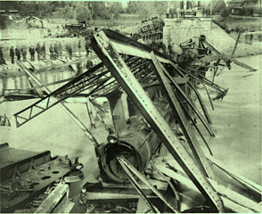
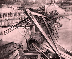
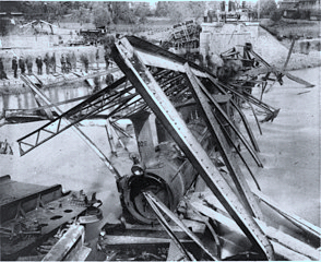
Or take the event that some bridge with a known fatal defect will collapse over the next day. Assume that it is judged to be a probability 0.6 event.

A rail bridge collapse in Münchenstein,
Switzerland, June 14, 1891.
https://en.wikipedia.org/wiki/File:Birs_1891_c.jpg
What do we mean by these two probability statements? When we try to give a similar explicit definition for probability as an answer, the problems start:
The probability of an event is ...
Just how is the "..." to be filled in. The modern literature has many different attempts. Here are three approaches. As you will see, none is entirely satisfactory.
These interpretations seek to identify something objective in the world that corresponds to probability. By "objective" we mean something that exists independently of we human subjects. Probabilities understood this way are sometimes called "chances" in philosophical writing. The simplest case is the die cast. To say that the cast of a 6 has probability 1/6 is to say that a 6 arises in roughly one sixths of the repeated casts:
...
Something like this seems like it should work out. The problem is that "roughly one sixth" is not precise enough to serve as a definition. Precisely what does "roughly" mean here? In any sequence of casts it can happen, with lower probability, that all the casts are 6's.
...
This can happen even though the probability of each individual six is still 1/6. We might imagine that everything works out if we just cast the die often enough. In the limit of infinitely many die casts, one sixth will be 6's. Even that is not quite right since there is a probability zero of all infinity of die casts being 6. Probability zero events are exceeding rare, but they are not impossible. Even in that exceedingly rare case, we would still say the probability of a six is 1/6.
The problem is worse for the case of the bridge collapse. What replaces the infinitely many casts of the die? Are we to imagine infinitely many identical bridges and ask how frequently they collapse? Or are we to consider infinitely many bridges just like the one in consideration in the aspects relevant to the probability of collapse? But if we cannot say what the probability of the collapse is, how do we know which those relevant aspects are?
 ...
...
An alternative approach understands assertions of probability to be about our beliefs, or more cautiously, about our beliefs when formed responsibly in the light of evidence. Probabilities understood this way are sometimes called "credences" in philosophical writing. That a bridge has a probability of collapse over the next day of 0.6 ultimately just means that we believe with an intensity of 0.6 that the bridge will collapse.

A great advantage of this approach is that we can give an operational definition for these probabilities-as-beliefs. We can recover a person's beliefs from their behaviors. Imagine that someone is willing to accept either side of a bet with 60 to 40 odds on the collapse of the bridge, then we would judge them to harbor a belief-probability of 0.6.
The disadvantage of this subjective interpretation is that the probability of a bridge collapse seems to be something other than merely our beliefs. Is it not an objective feature of the world, independent of what we may think or believe?
Another approach simply gives up on trying to complete the sentence, "The probability of an event is ..."
The probability of an event is ...
Instead, the approach asks us consider all the true statements that we can make about probabilities. They are additive measures. They can form conditional probabilities. They can be multiplied for independent events. And so on. We connect probabilities with frequencies with a version of the law of large numbers:
With probability one, the frequency of occurrence of a probability 0.6 outcome in infinitely many independent trials is 60%.
In none of these efforts do we ever say what probability is. This last statement about infinitely many trials does not do it. It begins with the words "With probability one..." That means that we already need to know what probability is before we can understand the statement.
The great advantage of this approach is that it licenses us just to keep doing what we have always done. We have at our disposal a sufficiently rich collection of truths containing the word "probability" so that we can continue to compute all our probabilistic results as before.
The disadvantage of this approach is the we remain unsure of what we have computed when we arrive at the result:
"The probability of a bridge collapse over the next day is 0.6."
What do we mean by probability in this statement?
The best attempt I know to solve this last problem uses what has been called "Cournot's principle." The principle tells us that, if some outcome has high probability close to one, then we should expect it to happen.
To use the principle, we convert the case of interest into one that has very high (or sometimes very low) probability. If some occurrence has a probability of 0.6, we would take that to mean that, if we were to repeat the trial very many times, we should expect about 60% successes.
The advantage of this approach is that comes quite close to how we think about probability in ordinary circumstances. How do we distinguish a probability 0.5 outcome from a probability 0.6 outcome? The first, we say, occurs 50% of the time on average; and the second 60% on average.
The disadvantage of this approach is that it depends on imprecise notions. We expect about 60% successes. We expect... This last "expect" is necessarily a notion outside of the probability theory. Otherwise we have not provided an independent meaning for probabilistic terms. But if it is outside the probability theory, just what does it mean? There is not independent theory of the nature of expecting provided by Cournot's principle.
Copyright, John D. Norton