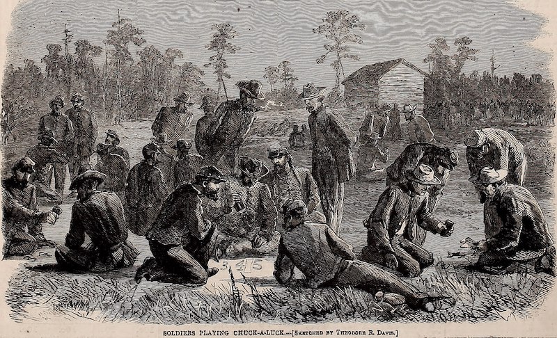
Soldiers playing chuck-a-luck in Harper's Weekly, 1865.
https://commons.wikimedia.org/wiki/File:Harper%27s_weekly_(1865)_(14784937143).jpg
| HPS 0628 | Paradox | |
Back to doc list
Paradoxes From Probability Theory: Expectations
John D. Norton
Department of History and Philosophy of Science
University of Pittsburgh
https://sites.pitt.edu/~jdnorton/jdnorton.html
Linked document: The Gambler's Ruin (pdf) (Word)
For a compact reminder of expectations in probability theory, see Probability Theory Refresher: Expected Value.
We have seen how attention to mutual exclusivity and independence in the probability calculus can correct our judgments about chance phenomena in surprising ways that seem paradoxical, initially. There are similar corrections deriving from the properties of expectations or expected values in the probability calculus. We shall see two of them here.
The first is the popular game of "chuck-a-luck" or "crown and anchor." A natural supposition that the game favors the player is refuted by computing the expectation.
The second is the extent to which a gambler is harmed by a slightly negative expectation. What is presumed to be a benign effect produces what is called in the probability literature, the "gambler's ruin."
When gambling games are simple, it is fairly easy to see whether they favor the gambler or not. Computing the expected value is likely unnecessary for most of us to see which game is fair and which is not. Things are not always so simple. Then computing the expected value can give useful information.
A game is known as chuck-a-luck in the US and related places; and as "crown and anchor" in England and related places. It is played with three dice. In the US they are numbered one to six. In England they have the four card suits, a crown and an anchor on their sides.
Soldiers playing chuck-a-luck in Harper's
Weekly, 1865.
https://commons.wikimedia.org/wiki/File:Harper%27s_weekly_(1865)_(14784937143).jpg
A player is invited to bet on one of the sides for
a fee of $1. In the US game, the player may choose any number. For
concreteness, let us say that is it a six  .
If one of the dice shows a six, the player is
paid a net of $1. If two
show, the player is paid that twice: a net of $2. If all three dice show a
a six , the player
is paid this $1 amount ten times: a net of $10.
.
If one of the dice shows a six, the player is
paid a net of $1. If two
show, the player is paid that twice: a net of $2. If all three dice show a
a six , the player
is paid this $1 amount ten times: a net of $10.
![]()
![]() +$1
+$1
![]() +$2
+$2
+$10
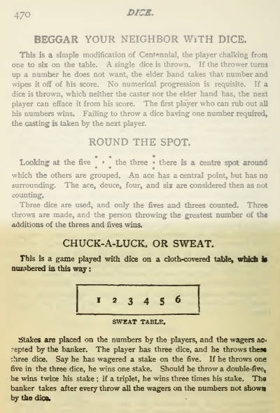
Here is a version of chuck-a-luck from
Hoyle's celebrated (1904) book of rules for games. This version
is less favorable to the player. It only requires a payment of $3 if all
three dice show the player's chosen number:
The game seems fair on cursory considerations. Players often reason as:
"There is a one in six chance of a six
on just one die. Since there are three dice, I get three opportunities of
a one in six chance. That is, there is a one in two chance of a win. So I
have even odds: an equal chance of winning $1 and of losing $1. But
wait... when a six
comes up on one die, there are still two others. And if any of those also
show a six , I win
there too. If all three, I get ten times as much! Thus the game favors me.
I get three ways of winning to the house's one."
Needless to say, this sort of reasoning is just what the house wants the player to think. In practice, the game is slightly favorable to the house. To see it, we need to pay attention to the outcome space. Its elements are outcomes of the form:
six
on the first die
and not on the
second and third
six
on the second die
and not on the the first and third
and so on.
We then need to compute the probabilities and then the expected value in this outcome space. Here is how the computation looks:
is merely 75/216 = 0.347, that is, roughly a third. An even odds bet on
just this outcome is clearly unfavorable.P(one six
only)
= P(six
on the first die
and not on the
second and third)
+ P(six
on the second die
and not on the the first and third)
+ P(six on the
third die
and not on the the first and second)
=(1/6)x(5/6)x(5/6)
+ (5/6)x(1/6)x(5/6)
+ (1/6)x(5/6)x(5/6)
= 3 x (1/6)x(5/6)x(5/6) = 75/216
Similar calculations give:
P(two sixes
only) = = 3 x (1/6)x(1/6)x(5/6) = 15/216
P(three sixes )
= (1/6)x(1/6)x(1/6) = 1/216
P(no sixes )
= (5/6)x(5/6)x(5/6) = 125/216
We can now combine these probabilities and compute:
Expected value
= P(one six
only) x $1
+ P(two sixes
only) x $2
+
P(three sixes ) x
$10 - P(no sixes )
x $1
=(75x$1 + 15x$2 + 1x$10 - 125x$1) / 216
= -$10/216
= -$0.0463
That is, the expected value is a net loss of -$0.0463. What this means is that in repeated playing of the game, the player loses an average of $0.0463 on each play.
This average loss is small enough that it is hard to notice behind the normal variations in wins and losses. If a player makes 100 plays, the player will on average only have lost $4.63. For the player, that is just the fee paid for the opportunity of 100 plays and the enticing chance of a big win. For the house, however, this small loss by the players, is a gain for the house. Over the longer term, these gains build and keep the game profitable for the house.
In a fair game, neither the gambler nor the house has any advantage. This fairness entails that the expected return to either on any play is zero. For if one--the house, for example--has a positive expectation, then the other--the gambler--must have a negative expectation. The house would then be favored only because the gambler is disfavored.
This means that gamblers should seek fair games in which their expectation on each play is zero. Of course if a gambler can find a game in which the gambler has a positive expectation, that would be the even better choice. However in practice this option is not offered in casinos unless by mistake. The realistic choice is between games, all of which have some negative expectation. The better choice is the game with the less negative expectation.

The casino at Monte Carlo
https://commons.wikimedia.org/wiki/File:The_Casino,_Monte_Carlo_-_panoramio_cropped.jpg
It is easy to imagine that a small negative expectation will not have much damaging effect. That this is mistaken is the principal conclusion to be drawn from the "gambler's ruin" problem.
To calibrate what we anticipate should happen, we first consider a simple fair game. The game play has two outcomes--red and black--each with probability 1/2. We could imagine that the outcomes arise from tossing a coin with red on one side and black on the other. The game pays a net of +$1 on red and -$1 on black.
 +$1 p
= 1/2
+$1 p
= 1/2
 -$1 p
= 1/2
-$1 p
= 1/2
The expected value of each play is
Expectation = +$1 x 1/2 + -$1 x 1/2 = 0
On each play, the gambler either wins or loses $1. It follows from the zero expectation that on average, with each play, the gambler gains or loses nothing.
The gambler approaches the game with an initial stake of $50 and plans to keep playing until the gambler's fortune has risen to $100 ("win"), that is, until it has doubled; or the gambler has lost the entire $50 stake, which is the "ruin" of the "gambler's ruin." The overall dynamic, as play proceeds, is for the gambler's fortune to rise and fall.
Here is a simulation of the changing fortunes of ten gamblers, each of whom play for 1,000 bets:

The chart illustrates the main features of the play.
Symmetry
While each gambler's fortune will move either up or down, there is no preferred direction. Overall the gambler's fortunes are as likely to rise and fall.
This lack of a preferred direction follows from the
symmetry of the game. If we switched the rules so that the gambler were to
lose $1 on a red outcome and gain $1 on a black outcome, then the dynamics
would remain the same. Thus the dynamics can show no preference for either
of the directions. This reversed game is the one that the house is
actually playing.
Probability of win or ruin
Because of the symmetry of the game, the chance of winning or of ruin are the same. If we assume that the gambler keeps playing until either happens, then their probabilities must sum to unity and be one half for each:
Pwin = Pruin =1/2
Duration of play
The gambler starts with a fortune of $50. As play proceeds the gambler's fortune will rise and fall. It will meandering around the average of $50, but gradually drift farther and farther away from it, until it has drifted to $100 (win) or $0 (ruin). In the simulation above only two of the gamblers have drifted far enough to halt play. One drifted to a win and the other to ruin.
We can ask how far the fortunes drift as play proceeds. The drift motion is a classic of stochastic processes, the so-called "random walk." For such processes the distance drifted on average follows a simple rule:
average drift is proportional to √(number of plays)
We are interested in how many plays are needed for a win or for ruin to arise. There is no single number since some games will end early and other late. However we can determine an expectation value for the number of games that leads to termination by inverting this drift estimate. In the inversion, the number of plays is proportional to (average drift)2.
More specifically, we seek how many plays are needed for the drift to extend to $50, either in a gain or a loss, for that marks the end of play. The inverted result tells us that the number of plays for termination is proportional to 502. A more precise analysis (given in the linked pdf) shows that the result is not just proportionality but equality:
Expected duration of play = 502 = 2,500 plays
The chart above only extends to 1,000 plays, which is well short of this expected duration. If it were to be extended, more of games would terminate by the expected duration of 2,500 plays. We would likely have to extend well beyond this value of 2,500 in order to find all the games terminating.
There is something close to this fair red/black game in the game of roulette, as it is offered traditionally in casinos. In the American version, there is a wheel with slots numbered 1 to 36 and two slots numbered 0 and 00. The slots numbered 1 to 36 are divided into 18 red and 18 black slots. Gamblers can bet with equal odds on red or black; or on a low number 1-18, or a high number 19-36; or an even number or an odd number. A bet on any of these loses, however, if either the 0 or 00 arises.

Outer rim from
https://commons.wikimedia.org/wiki/File:Basic_roulette_wheel.svg
Since each number arises with the same probability and there are 36+2=38 of them, a bet on red has the following probabilities and payoffs:
RED
+$1 p
= 18/38
BLACK
or 0 or 00
-$1 p = 20/38
The probabilities and payoffs are switched for a bet on black.
Since 18/38 = 9/19 = 0.474 < 1/2, the game is unfair. The expectation on a bet of $1 on either red or black is
Expectation (red) = Expectation (black)
= $1 x
18/38 - $1 x 20/38 = -$(2/38) = -$(1/19) = -$0.0526
This is a small, negative expectation. It is merely about 5% of the $1 bet. One might imagine that a such small negative expectation would not alter the dynamics of play. That is not so. The chart below shows a simulation of ten gamblers repeatedly making $1 bets on red at roulette. As before, they start with a stake of $50 and continue to play until their fortune has risen to $100 (win); or it has fallen to zero (ruin):

Over the same 1,000 plays simulated for the fair game above, the dynamics are quite different. The fortunes of the gamblers do drift, but they all drift in a downward direction.
We can compare this behavior further with that of the fair game:
Symmetry
The symmetry of the fair game is lost. The gamblers' fortunes all drift downward towards ruin. If we reverse the payoffs above, we have how the house experiences the game. If there is a black or 0 or 00, the house wins $1, with probability 20/38; and if there is a red, the house loses, $1 with probability 18/38. The house has a positive expectation in each play of +$0.0526. The house's fortune, if charted, would show an upward drift.
Probability of win or ruin
The probability of ruin in the fair game is 1/2. The probability of ruin in this unfair roulette game is so close to 1 that the difference is indiscernible in ordinary play. That is, any gambler playing this game with this strategy will almost certainly face ruin. A precise calculation of the probability of ruin is given in the linked pdf. The formula uses the ratio of the probabilities of a loss and a win in a single play:
Probability of loss / probability of win
=
(20/38) / (18/38) = 10/9
This figure of 10/9 is then used in general formula:
Probability of ruin
= [ (10/9)100 - (10/9)50 ]
/ [ (10/9)100 - 1 ]
= [37,649 - 194] /
[37,649 - 1 ] = 0.9949
A probability of ruin of 0.9949 is very close to one, certainty. It is roughly
995/1000 = 1 - 5/1000 = 1 - 1/200 = 199/200
The means that on average, if 200 gamblers play with this strategy, 199 of them will be ruined and only 1 will win. This dismal fate is reflected in the chart above. Over the 1,000 plays simulated, 8 of the 10 gamblers were ruined. The remaining two played on. One was already close to ruin and second has less than the starting stake.
Duration of play
The simulation charted above also suggests that the expected duration of play is shorter than that of the fair game. In the simulated fair game, only two gamblers of ten had terminated play in 1,000 plays. In this unfair game, in 1,000 plays, 8 of 10 gamblers have been ruined.
The full analysis given in the linked pdf shows that the expected duration of play can be easily approximated in cases like this in which the probability of ruin in near certain. We start with the stake of $50 and allow that, with each play, there is an expected loss of $1/19, as calculated above. The expected duration of play is the number of plays needed for the accumulated losses of $1/19 per play to exhaust the initial stake. That is:
Expected duration of play
= Initial stake / expected loss per play
= 50 / (1/19) = 950
This expected duration of play of 950 is less than half the expected duration of play of the fair game of 2,500. It tells us that the near assured ruin in the unfair game will come more swiftly than any ruin in the fair game.
These last sums make matters look bad for a gambler playing an unfavorable game. If we assume that the gambler makes many smaller wagers, as opposed to a few larger ones, then we can see that situation is even worse than it seems so far.
If the gambler plays a fair game, then the gambler can skew the chances of winning in the gambler's favor by risking a larger stake:
If
the gambler seeks to win 100 risking a stake of 100, the probability of a
win is 100 / (100 + 100) = 1/2.
If the gambler seeks to win 100 risking a stake of 900, the probability of
a win is
900 / (900 + 100) = 9/10
One might then imagine that in, an unfair game, the effect of a negative expectation can be mitigated by playing with a larger stake. The intuition is that if one risks more, one should have a greater chance of gaining.
This intuition fails in the case of a gambler in an unfavorable game who plays with many smaller bets. For then, as is shown in the linked pdf, the formula for the probability of ruin simplifies. For the case of roulette, it simplifies to
Probability of ruin
= 1 - (10/9)(-target
gain amount)
Here the "target gain amount" is the amount that the gambler seeks to gain when the gambler is willing to risk the entire stake to secure it. It is measured in the size of the bets made as units.
If the gambler wishes to gain $50 in red-black bets on roulette, betting in small units of $1, then the above formula gives us:
Probability of ruin
= 1 - (10/9)-50
= 1 - 0.005154 = 0.9948
This agrees with the probability of ruin already computed above when the stake was 50. What we now see is that this dismal probability will be same, no matter how large we make the stake:
Probability of ruin = 0.9948 if the stake is 50 or 100 or 500 or 1,000 or...
It is not too hard to grasp intuitively why this is so. If the gambler is to win the targeted amount, it must happen early in the play before much of the stake has been exposed to loss. Once that early win has failed, the gambler will have cut deeply enough in the original stake that recovery ceases to be possible. The gambler will just continue to lose and lose and lose, exhausting any stake, no matter how large.
A simple mechanical analogy might help clarify the difference between the two cases. Imagine that we have seven small cups in a row on a board. We put a pea in the central cup and will shake the cups and board. The walls between the cups are low so that the pea can bounce between the cups. The walls on the other sides are high so that the pea can only bounce between adjacent cups. There are two, additional destination cups at the left "L" and right "R" ends of the two

Keeping the board horizontal, we shake the board and cups up and down so that the pea jumps around between the cups. There is an equal chance that the pea will jump to the right or to the left. If we keep shaking long enough, the pea's drifting back and forth between the cups will eventually lead it to escape to either the left or right destination cup. From the symmetry of the arrangement, there is an equal probability that the pea ends up in either left or right cup. (This case corresponds to the fair game.)

Now imagine that we incline the board and cups slightly to the right and repeat the shaking. The slight incline means that the pea is slightly more likely to jump to a cup on its right than on its left. Over the course of many shakings, the pea will migrate preferentially to the right and end up in the right destination cup. (This case corresponds to the unfair game.)

While the inclination of the board and cups may be small, in many bounces, it is enough to favor a rightward drift quite strongly. Correspondingly, a small negative expectation in the red bets in roulette is enough to favor quite strongly a downward drift in the gambler's fortune.
"If you must"? It does not take much acquaintance with probability theory to see that casino gambling is a poor idea for someone interested in turning a profit or just breaking even. What the gambler's ruin problem shows is that gambling by the strategy sketched above is not just a poor idea, but a very poor idea. That ruin is assured for this strategy in the unfair game is surely surprising and even paradoxical in the sense of a strikingly unexpected result.
The analysis, however, does suggest an alternative strategy that gamblers can use to mitigate the approaching ruin:
Make the largest bet you can.
That is, if you have a stake of $50, bet it all at once. As before, the bet has a negative expectation of -$50x(1/19) = -$2.63. However the prospect of ruin is greatly reduced. We have
Probability (win $50, fortune to $100) =
18/38 = 0.47
Probability (lose $50, ruin)
= 20/38 = 0.53
This strategy has the same result as the single $1 bet strategy: the game ends with the gambler's fortune rising to $100 or falling to $0. However now the probability of ruin is much less. It is just over 1/2.
That this shift in strategy makes such a big difference is something peculiar to the unfair game. In the fair game, the probability of a win or a loss is always 1/2, independently of whether the gambler makes many single $1 bets, bets the entire stake of $50 all at once or has some combination in between. That this is so, follows from the symmetry of the game. As long as the gambler plays so that the only outcomes are a win or ruin, the probabilities will always be 1/2.
It may seem puzzling that the probability of ruin can be so easily reduced in an unfair game by making the largest bets possible. That it is puzzling may come from the following (flawed) reasoning:
"If
I bet all my stake of $50 at once, my expectation is just -$50x(1/19) =
-$2.63.
If I divide my stake into 50 single $1 bets, then my expectation in each
is -$(1/19). But there are 50 bets, so my overall expectation is the same
-50x$(1/19) = -$2.63.
Thus there should be no difference in the effect of the negative
expectation in the two cases."
The false assumption is in the second inference "... there are 50 bets..." There are not 50 bets, but very many more in the chosen strategy. We saw above that the expected duration of play is 950 plays. That is, the gambler will actually place 950 bets on average, before ruin, and in each of these incur a negative expectation of -$(1/19).
As before, the accumulated negative expectation is -950x$(1/19) = -$50, which erases the gambler's initial stake.
We have seen that a game with negative expectation for the gambler is unfavorable and that ruin is likely. If however the gambler can somehow secure a game with a positive expectation, then the tables are turned. The gambler now has the advantage. Let us explore how the gambler might exploit this advantage. We can re-use the results concerning the gambler's ruin. They are just reversed to form the gambler's revenge.
Games with positive expectations for the gambler are hard to find. What casino would willingly offer a game in which the gambler and not the casino has the advantage? A rare case in which this is supposed to happen is the card game of blackjack. In the game, the gambler and a dealer, representing the casino, seek the most favorable hand in cards drawn from several, well-shuffled decks. If the game is played well by the gambler, the casino has only a slight edge. Each gambler's bet has a negative expectation of less than 0.5%.
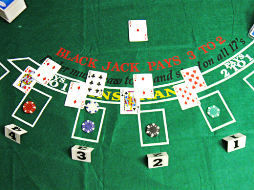
https://commons.wikimedia.org/wiki/File:Blackjack_game_1.JPG
That slight advantage persists as long as gamblers play as if all the cards have an equal chance of being drawn from the decks. As cards are drawn from the deck, however, the actual probability of different cards being drawn changes. For example, there are four aces in a single deck of 52 cards. Initially, there is a probability of 4/52 = 1/13 of drawing an ace.


If however, in play, none of the the first ten cards drawn is an ace, then the probability of an ace increases. There are still 4 aces in the remaining deck of 42 cards. So the probability of an ace is 4/42 = 1/10.5 > 1/13.
Card counters in blackjack keep track of the cards that have been drawn from the decks. Their goal is to wait until fewer than average high cards have been drawn. These high cards are ten, jack, queen, king and ace of any suit. Then the probability of these high cards being drawn increases. In that circumstance, a careful gambler now has an advantage over the casino.
Overall, the common estimate is that a competent card counter at blackjack can gain a positive expectation of 1%. That is, the expectation on bets of $100 is +$1. This positive expectation favors the gambler. However the advantage is meager compared with the advantage of the casino in other games. We saw above that a gambler in roulette has a negative expectation of 5.26%.
Set aside the details of card counting in blackjack. There are many complications to which we cannot attend here. Let us just assume that somehow a gambler has been able to secure a game in which the gambler has a positive expectation of 1% on each bet. How best can the gambler exploit this advantage?
Compare this new gambler's situation with what we saw for gamblers in games with unfavorable, negative expectations:
Games
with negative expectations:
Best strategy: Play with as few, large bets as possible.
Worst strategy: Play with as many, small bets as possible.
When playing games with a positive expectation, the
gambler has taken on the position of the casino. These strategy
recommendations are reversed.
Games
with positive expectations:
Worst strategy: Play with as few, large bets as possible.
Best strategy: Play with as many, small bets as possible.
The good news for the gambler
With the tables turned, the gambler is now in the happy position that what was "ruin" is now a "win." The strategies are now reversed. The gambler should not now make a small number of big bets since that will reduce the probability of winning. The probability of winning is now large if the gambler plays with many small bets.
The approximate formula above for this case of many small bets in an unfavorable game of roulette was:
Negative expectations
Probability of ruin
= 1 - (10/9)(-target
gain amount)
With the tables turned:
"ruin" becomes "win"
"target gain amount" becomes "stake"
Apply this to case of the positive expectation of 1%. The ratio of 10/9 in roulette is replaced by 101/99 and the new formula is:
Positive expectations
Probability of win
= 1 - (101/99)(-stake)
We can calculate a few values:
Probability of win (stake = 50) is 1 - (101/99)(-50)
= 0.6321
Probability of win (stake = 100) is 1 - (101/99)(-100) =
0.8647
Probability of win (stake = 500) is 1 - (101/99)(-500) =
0.999955
The best part of these calculations is that the target gain amount does not enter into the probability. Fix the stakes the gambler is willing to risk and choose any target gain amount, then the above probabilities apply!
This too-good-to-be-true result is the reverse of the corresponding result in unfair games: that the gambler will continue to lose indefinitely if an easy win has not occurred. Now the gambler will continue to win indefinitely, as long as an early loss did not occur.
The bad news for the gambler
So far, the situation does have a too-good-to-be-true feel to it. There is a catch. To secure these favorable probabilities, the gambler must play with many small bets. That means that the duration of play will be long.
Assume that the player makes bets in units of $100. The expected gain on each is 1% = $1. How long would it take to earn $10,000 = 100 betting units? Using the expected gain to estimate the duration of play, the number of bets needed is roughly 100/0.01 = 10,000. If the gambler can make one bet each minute that translates into:
10,000 minutes = 167 hours = 20.8 eight hour days
Thus, what matters most to winning in a game with positive expectation is not the size of the stake the gambler can assemble. It is simply the stamina of the gambler to keep betting and winning with small bets. When everything is working perfectly in the scenario depicted, the gambler will make roughly $60 per hour.
While these last calculations do indicate that a card counter with stamina has a real prospect of profiting at blackjack in a casino, it is worth stepping back and asking just how realistic those expectations are.
Casinos are businesses. They exist to make profits, not to benefit gamblers. And make profits they do. If card counting at blackjack was a realistic way for gamblers to make assured profits, they would also be assured losses for the casinos. In that case, the casinos would not offer the game. Or the casinos would implement small changes in the gaming protocol that would defeat card counting.
That casinos continue to offer the game of blackjack is the surest indication that card counting is not so lucrative. Presumably the stamina needed for very long gambling sessions, while accurately counting cards, is beyond most casual gamblers. But the idea that a casual player might beat the casino is, no doubt, just the sort of enticement casinos need to draw in players. The more who come and try and fail, the more profit the casino makes.
Perhaps there are some highly disciplined card counters with the stamina to play long enough to win. They are easily identified and casinos can ask them to leave. There are videos online of just such ejections. We might guess that these videos are useful to the casinos. They reassure casual gamblers that card counting works and thus help to entice these gamblers into the casino. And we might guess that they are useful to the stymied card counters. They can then use them as credentials in advertisements for services in which they offer to train clients to card count.
May 5, 2022.
December 24, 2022.
Copyright, John D. Norton