The passive cable equation

Information flows in the nervous system from the soma to the axon and then to the dendrites. In most models, the dendrites are regarded as being passive electrical cables. In this section, the cable equation is derived, steady state cable properties are studied and total input resistance of a cell is defined.

  

Figure 2: Cable broken up into discrete segments

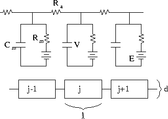We will model the cable as a continuous piece of membrane that consists of a simple RC circuit coupled with an axial resistance that is determined by the properties of the axoplasm. Figure 2 shows a piece of a cable broken into small parts. From this figure, we obtain the following equations  

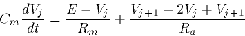$$C_m\frac{dV_j}{dt} = \frac{E-V_j}{R_m} + \frac{V_{j+1}-2V_j+V_{j+1}}{R_a}$$ (7)

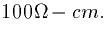We have introduced a new quantity, R_a which is the axial resistance. This as you would guess depends on the geometry of the cable, in this case, the diameter, d and the length, $\ell.$ As with the membrane resistance, there is also a material constant, R_A associated with any given cable. This is measured in $\Omega-cm$.A typical value is $100\Omega-cm.$ As anyone who has ever put a stereo will attest, the resistance along a cable is proportional to its length and inversely proportional to the cross-sectional area (the fatter the cable, the less resistance) thus we have the following (using our definitions above)

We plug these into (7), let $x=j\ell$ define distance along the cable, and then take the limit as $\ell\to0$ to obtain the continuum equation for the cable:  

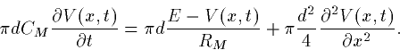$$\pi d C_M \frac{\partial V(x,t)}{\partial t} = \pi d \frac{E... ...{R_M} +\pi \frac{d^2}{4} \frac{\partial^2V(x,t)}{\partial x^2}.$$ (8)

We multiply both sides by $R_M/\pi d$ and obtain the following equation:  

$$\tau_m \frac{\partial V}{\partial t} = E-V + \lambda^2\frac{\partial^2V}{\partial x^2}$$ (9)

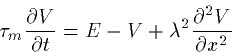
where $\tau_m$ is the time constant R_M C_M and  

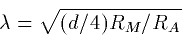$$\lambda =\sqrt{(d/4)R_M/R_A}$$ (10)

is called the space constant of the cable. The space constant depends on the diameter while the time constant depends only on the material constants. Using $R_M=10000\Omega {cm}^2$ and $R_A=100\Omega cm$ we obtain

$$\lambda= \sqrt{25d}$$

so if the dendrite has a diameter of, say, 10 microns, or 0.001 centimeters, the space constant is 0.07 centimeters or 0.7 mm. The space constant determines how quickly the potential decays down the cable.

An alternate derivation is given by Segev in the Book of GENESIS. The longitudinal current, I_i is given by the following:  

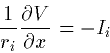$$\frac{1}{r_i}\frac{\partial V}{\partial x} = -I_i$$ (11)

where r_i is the cytoplasmic resistivity as resistance per unit length along the cable. This is just $4R_A/(\pi d^2).$