Consider in Figure 7
the I-interval between A and D.
There is a stable rest state around -35 mV and a stable
(more depolarized) limit cycle.
Suppose the current I slowly varies back and forth across
this interval.
Then because of the bistability, it is easy
to see how a hysteresis loop is formed in which the membrane is
alternately at rest and alternately firing repetitively. This
provides a simple mechanism, and geometric interpretation,
for square-wave bursting. However, since
the current I is externally imposed, this is forced rather than
autonomous bursting.
To achieve the latter, one could (as in [31])
redefine I as a dynamic
dependent variable in such a way that I
decreases when the membrane is depolarized and
firing repetitively, and I increases when the membrane is resting.
Although artificial, this example
demonstrates the basic principle that (very) slow negative feedback
together with hysteresis in the fast dynamics underlie
square-wave bursting.
Many different ionic current mechanisms could likewise produce
the slow negative feedback.
For further illustration we employ a calcium-dependent potassium
current, analogous to that studied by others
(see [36]).
We assume the current activates instantaneously in response to
calcium
and that the calcium handling dynamics are slow. Thus, we add
to (6) the current  given by
where  is the maximal conductance for this current and z is the gating
variable with a Hill-like dependence
on Ca (the near-membrane calcium concentration scaled by
its dissociation constant for activating the gate,
is the maximal conductance for this current and z is the gating
variable with a Hill-like dependence
on Ca (the near-membrane calcium concentration scaled by
its dissociation constant for activating the gate,  ):
):
(For simplicity, we set the Hill exponent p=1, although this is not required.) The balance equation for Ca is:
where the parameter  is for converting current into a concentration
flux and involves the ratio of the cell's surface area to
the calcium compartment's volume.
The parameter
is for converting current into a concentration
flux and involves the ratio of the cell's surface area to
the calcium compartment's volume.
The parameter  is a product of the calcium removal rate
and the ratio of free to total calcium in the cell. Since calcium is
highly buffered,
is a product of the calcium removal rate
and the ratio of free to total calcium in the cell. Since calcium is
highly buffered,  is small
so that the calcium dynamics is slow.
This is a greatly simplified model, for example,
one could have more complicated
calcium handling, including diffusion of calcium in the cytoplasm,
nonlinear removal of calcium by pumps/exchangers, perhaps even
release of calcium from intracellular pools.
If the conductance
is small
so that the calcium dynamics is slow.
This is a greatly simplified model, for example,
one could have more complicated
calcium handling, including diffusion of calcium in the cytoplasm,
nonlinear removal of calcium by pumps/exchangers, perhaps even
release of calcium from intracellular pools.
If the conductance  of
this outward current is large, the membrane is hyperpolarized
and if it is small, then the membrane can fire. Thus, when a
bifurcation curve is drawn as a function of this conductance, it is
reversed from that of Figure 7 which plots the behavior as a function
of an inward current. When the membrane is firing, intracellular
calcium slowly accumulates, turning
on this outward conductance and thereby terminating
the firing. Figure 9a shows a bursting solution to the
three variable model, eqns. 4-6 coupled with the slow
calcium dynamics, eqn. 22.
of
this outward current is large, the membrane is hyperpolarized
and if it is small, then the membrane can fire. Thus, when a
bifurcation curve is drawn as a function of this conductance, it is
reversed from that of Figure 7 which plots the behavior as a function
of an inward current. When the membrane is firing, intracellular
calcium slowly accumulates, turning
on this outward conductance and thereby terminating
the firing. Figure 9a shows a bursting solution to the
three variable model, eqns. 4-6 coupled with the slow
calcium dynamics, eqn. 22.
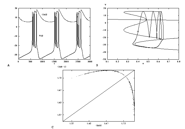
(A,B) Run this to see the projection in the z-V plane. Plot
V versus t. Change the current, I and the
conductance of the AHP current, gkca to see what happens.
When is there no longer bursting? Plot the calcium as a function of
time. (C) Run the simulation longer (say, 4500)
with I=45, gkca=0.25 and
now changing Ca0=12. There is no longer bursting but the
repetitive firing is not regular. Now, if you want, you can look at
this chaotic behavior. Compute the Poincare map
as follows.
Set V=-22.63, w=0.018, ca=18.53 as
initial data; ca0=12 . Now set the total simulation time to
50000 and set Dt=0.25 From the (nUmerics) menu, choose
(Poincare map) (Section) The following should be filled in:
While still in the numerics menu, choose (rUelle plot) and make the
X-axis shift 1 and the rest 0. Escape to the main menu.
Change the (Viewaxes) (2D) so that Ca is on both axes and window
the view between 19 and 21 on both axes. Finally, uses (Graphic
stuff) (Edit Curve) to edit curve 0 and change the linetype form 1 to
0. Now run the integrator by choosing (Initconds) (Go) (It
will take a while.) You will see a diagonal line of points plotted. If
you get bored, type (Esc) to stop. Choose (Restore) and you will see
a cap map like Figure 9C. You have computed a Poincare map, plotting
the values of calcium every time the potential decreases through 0.
Projecting the solution onto the z-V plane, where z is
defined in eq. 21, shows (Figure 9B) how the burst's trajectory
slowly tracks the
attracting branches of the fast subsystem. Rapid transitions occur
when the branches terminate at bifurcation points and turning points.
We note that any number of alternate mechanisms could provide the
slow negative feedback for bursting including a slow gating kinetics
for z with fast calcium handling, or slow inactivation of
 , driven by V or Ca.


