Chaos ....
Chaos is a phenonenon with many meanings depending on whom you ask.
For the purpose of this tutorial, I will say that a system is
chaotic if there is sensitive dependence on initial
conditions. That is, if I start with two initial conditions that
are very close to each other, then their difference will diverge
exponentially in time.
For discrete dynamical systems, it is possible to get chaotic
behavior with a one-dimensional map, as you saw with the standard map. For continuous systems,
the usual model for chaos is the Lorenz
attractor but the mechanism through which chaos occurs for this
model is somewhat difficult to explain.
When the linearization of a system about an equilibrium has a zero
eigenvalue for some set of parameters, this is a sign that perhaps new
solutions may exist for nearby sets of parameters. If the zero
eigenvalue is simple, then normal form analysis can be
applied to reduce the system to a one-dimensional dynamical system.
The dynamics of this one-dimensional system describes the behavior of
the full system. More complicated equations arise if the zero
eigenvalue is not simple. In the remainder of this tutorial, we
examine an equation that arises when the linearized system has a
triple zero eigenvalue that is geometrically simple. This means
that the characteristic polynomial starts with cubic terms.
The Jordan canonical form for the three-dimensional subspace with this
degeneracy is:

Since the characteristic polynomial has a triple degeneracy, we need
three free parameters to "unfold" this triple zero eigenvalue. Thus,
we will study the differential equation:

Notice that there is only one nonlinear term, a quadratic. Also note
that if the three parameters mu,nu,gamma are set to zero,
the linearized system is J.
A detailed analysis of this equation is beyond the scope of the
tutorial. However, we can explore the dynamics letting one parameter,
say , gamma vary. Thus, we fix q=2,nu=2,mu=1
and let gamma be our principle parameter.
Clearly (x,y,z)=(0,0,0) is always a solution, so we will
study stability and bifurcation of this. The easiest way to do this
is to use AUTO. (The stability of the fixed
point could be done analytically using the Routh-Hurwitz criterion,
but any other analysis is best doen numerically, even for this simple
system.)
Get the AUTO window up by clicking (File) (Auto). Within AUTO, do
the following:
- Click (Axes) (Hi Lo) and set
- Main Parm gamma
- Xmin 0
- Ymin -3
- Xmax 4
- Ymax 3
and click (Ok)
- Click (Numerics) and set
- Dsmin .0001
- Dsmax .1
- Par Min 0
- Par Max 3.75
- Norm Min 0.0
- Norm Max 50
and click (Ok)
- Click (Run) (Steady State)
You will see a line travel across the screen indicating the zero
steady state. It loses stability at gamma=2 Click (Grab)
and move the cross until Label 2 is reached. (Just click (Tab) to go
there quickly.) You will see that the type of point is HB
meaning a Hopf bifurcation has occurred.
- Click (Enter) to accept this
point and then click (Run) (Periodic) to compute the periodic solution
that comes from the point. Note the solution is stable (filled
circles) but loses stability.
- Click (Grab) and (Tab) 3 times until label 4 appears in the info
window in the AUTO window. Note it appears at gamma=3.126
and that its type is PD This indicates a period doubling
bifurcation which means that the basic limit cycle loses
stability and a new cycle arises that has twice the period. Click
(Enter) to accept this point.
- Click (Run) and (Doubling) to compute the branch of period two
solutions. This extends for a bit and itself becomes unstable through
yet another period doubling bifurcation. When
AUTO has finished the calculation, click on (Grab) and hit (Tab) 5
times to get the next period doubling point. It is Label 6 at
gamma=3.357
- Click (Enter) to accept this and then click (Run)
(Doubling) once again. This branch also becomes unstable at a period
doubling point for gamma=3.412.
We have found three period doublings. This is a classic scenario for
the onset of chaotic behavior: the period doubling cascade.
These calculations can be continued, but it would take a while, so we
will stop the continuation here.
Before continuing on, lets look at some of these solutions. We will
look at the limit cycles at the three points of instability.
- Click (Grab) and click (Tab) until label 4 appears and click
(Enter). Click (File) (Import Orbit). This loads this orbit into the
Data Browser so you can look at it.
- In the XPP main window, click (Viewaxes) (3d). Set the following
parameters:
- X-axis X
- Y-axis Y
- Z-axis Z
- Xlabel X
- Ylabel Y
- Zlabel Z
Ignore all the other stuff!! Click (Ok). Click on (Window) (Fit) to let XPP figure out the
window dimensions. The
orbit will be plotted in three-dimensions.
Freeze this curve with some color, e.g.color 7. (If you don't
remember how to freeze a curve, see
the first tutorial.
Go back to AUTO and get the next period doubling point, Label 6
using (Grab) and (Tab). Click (File) (Import Orbit) again. Then in
the XPP main window click (Window) (Fit) and freeze this curve with a
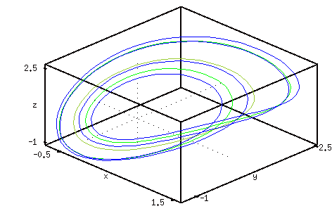
different color. Note how it loops around the phasespace twice. Its
period is roughly twice the other orbit's.
Repeat this for the third period doubling point (Label 8) and freeze
it with still another color. You will see that it loops around the
phase-space 4 times! You should have a picture that looks like:

Just for fun, click on (3d-params) in the main XPP window and change
Phi, Theta to rotate the three-d plot. You can actually
make a movie by rotating and then using
the Kinescope command. As this sometimes causes trouble on the
X-server, I won't officially do it here, but you can fool around at
your discretion.
In the previous section, we saw that there was an apparent period
doubling cascade. This is a classic scenario and sometimes "at the
end" of the cascade, there is a regime in parameter space where
chaotic behavior can occur. Before continuing go into the
AUTO window and click on (File) (Reset Diagram) and answer (Yes) so we
don't forget and leave AUTO junk all over the disk.
Click on (Graphic stuff) (Freeze) (Remove all) to get rid of all the
frozen curves and set the angles Phi,Theta back to 45 using
the (3d-params) command. Go into the (nUmerics) menu and set (Total)
to 150. (Escape) back to XPP main and set the parameter
gamma=3.5. Click (I)(G) to integrate. When done, click (W) (F)
to automatically fit the window to the data.
You should see a banded surface that is twisted like a Mobius strip.
This is chaotic attractor. To see it is chaotic, click on (Xi
vs T) to plot Z as a function of t. Click on (I) (N) and put the
following initial conditions in:
Freeze this curve with some nonzero color. Now, click (I) (N) again
and use the following initial data:
Window the graph so that the x-axis
goes from 100 to 150 and the y-axis goes from -1.5 to 3.5. Note thjat
the curves are quite different; small bumps and large bumps are
switched and so on. This shows sensitive dependence on initial
conditions the hallmark of a chaotic system. We changed the
fourth decimal place of an initial condition and the trajectory
changed completely after some time. What this says is that the
trajectories diverge exponentially in time. The rate of this
divergence is called the maximal Liapunov exponent. Stable
fixed points have a negative maximal Liapunov exponent, stable perioidic
orbits have a zero maximal Lyapunov exponent and chaotic orbits
have a positive maximal Lyapunov exponent.
Often in chaotic systems, a great deal can be learned by computing a
Poincare section. We will compute the section through X=0 as
it is clear that at every cycle, X passes through zero. (To
see this plot X vs t .) We will need to compute for a longer
period of time.
With this knowledge, you should close the continuous ODE file and fire
up the discrete map approximation.
If you haven't already, fire up the quadratic approximation to the
Poincare map of the dynamical system. Click on (nUmerics) and change
Total to 2000 and Method to (Discrete). (Escape) to
the main menu and edit the curve so
that the Linetype is 0 and we plot dots. Change the view to
plot Z on both axes as we will be using the Ruelle plots to
look at things. Integrate the
equations by clicking (I) (G). Click (W) (F) to fit the window to the
data. You will see a diagonal line. Then use the (G) (F) (F) to
freeze this diagonal.
You can keep all the defaults and just click on (Ok).
Now we will look for periodic points of different periods. A
point is k- periodic if Z(n)=Z(n-k) and Z(n) != Z(n-l) if l
< k thus, we need to
shift the x-axis by different amounts and look at the intersections
with the diagonal line.
- First we look for period 1 or fixed points of
the map. Click (nUmerics) (rUelle) and shift the x-axis by
1. (Esc) to the main menu and click (Restore). Note there is one
intersection and it is at about Z=2.43. The slope at the
intersection is greater than 1 in magnitude so it is unstable.
- Now look for period 2 points, by repeating the above and shifting
the x-axis by 2 instead. Note the appearance of two additional
intersections as well as the original fixed point. (Fixed points are
trivially periodic of all periods.)
- Try to find fixed points of period 3,4,5. Are there any? Be
careful that you don't mistake the fixed point for a higher period
point.
- Integrate for a total of 4000 and then look for higher period
points that are not powers of 2. I think there is are period 10,11
points. The resolution is bad for much higher than 11.
The existence of many unstable periodic points is often a hallmark of
chaotic behavior. As we mentioned previously,
another hallmark of chaos is sensitivity to initial conditions. For a
one-dimensional map, this is easy to quantify. We need to compute the
maximal Liapunov exponent:

where f'(xn) is the derivative of the map evaluated at the
nth iterate.
Since the log of the product is the sum of the logs
we can write this as the limit of an iteration. Close the above XPP
file and fire up the XPP file for
computing this. The source for this
is worth looking at to see how I did it. Basically, I compute
the iterate and then divide by the number of iterates (kept in the
t variable as an auxiliary variable
lexp.
Click on (View axes) (2d) and set the Y-axis to be lexp .
Set the dimensions so that the Y-axis runs between -1 and 1
and the X-axis runs between 0 and 2000. Click (Ok) and then
go into the (nUmerics) menu, set Total= 2000,
Bounds=1000, and Method= (D)iscrete. (Esc) back to the
main window and click (I) (G) to integrate the equations. You should
see a curve that rises and then flattens out at about .332. This is
the Lyapunov exponent and since it is positive, there is good evidence
that the system is chaotic.

References


 Table of Contents
 Main Menu Items
 ODE Files and Examples
 Numerics Menu
 File Menu
 Freeze Menu
 AUTO Menu
 Data Browser
 I/O and Hardcopy
 XPP Basics
 Nonlinear ODEs
 Two-dimensions
 Three-dimensions
and Beyond
 Phase Equations
 Chaos
Chaos