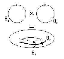
We have considered planar dynamical systems and if you have done the homework, you have explored some aspects of homoclinic orbits, bifurcations, and stability. The appearance of limit cycles through Hopf bifurcations, etc, is not restricted to planar systems. For example, an analysis similar to what we did with the Morris-Lecar model can be done with the Hodgkin-Huxley equations a 4 dimensional dynamical system. In this part of the tutorial, we will explore some other features of XPP. We will see how to use XPP to find the phase interaction function for weakly coupled oscillators. We will also study period doubling bifurcations, Poincare sections, and discrete dynamical systems. This is where we generally have to rely most heavily on numerical methods.

XPP has several useful features for dealing with I show some of the features that XPP has for dealing with these phase equations.
The main task at hand is to compute the phase interaction function. XPP gives you a very powerful tool for numerically computing the phase interaction function. But, first, to understand how to use this feature in XPP, I must once again go into math mode.
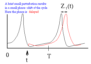
Suppose we have a system that is zipping along nicely on its limit cycle. Then at a particular phase in its cycle, we perturb one of the component quantities. This results in a small timing change in the oscillator, a phase shift.

The phase shift that results will depend on both the component of the limit cycle that was perturbed and the time in the cycle at which the perturbation occured. In the limit that the perturbations become infinitesimally small, this phase shift function tends to a computable vector quantity called the adjoint or response function. Each component of the adjoint gives the phase shift that results from administering a perturbation of the corresponding component in the limit cycle at the corresponding time of its cycle. Call this function Z(t). If the basic limit cycle in n dimensional so is Z(t).
Suppose we couple two identical oscillators X1'=F(X1) and X2'=F(X2) with weak coupling epsilon G1(X2,X1) :

Then, the interaction function which depends only on the phase-difference is computed by averaging the effect of the coupling with the response function or adjoint:

With this bit of stuff out of the way, it is clear what has to be done. After computing a limit cycle, the adjoint must be computed. Then the average of this must be computed. XPP provides simple steps for doing that which we will illustrate by starting with the Morris-Lecar equations and adding a synapse function which will serve to define a synaptic activity.

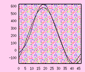
Having fired up XPP, we can integrate the equations several times to get on a nice limit cycle. Click (U)(T) to set the total integration time to 46.9 which is about the period. The idea is to get just one period of the limit cycle in the browser. Click (D) to set DeltaT to 0.1 which will speed things up a bit. Click (Esc) to get back to the main menu and then click (I) (G) to integrate the equations. In the ode file I have set the initial data on the limit cycle. Click (X) and type in V to plot the voltage versus time. Click (I)(L) twice to integrate the equations twice more strating at the values the previous integration left them. The graphs should almost superimpose showing you have a good estimate of the period. ( NOTE: How did I find the period? Here is how I do it: Integrate for a while to get several periods. Then use the data viewer to find the times between peaks of the voltage and use this as the period.)
Now we are ready to compute the response function. Click (U) (A) to bring up the adjoint/averaging menu. This menu allows you to compute the response function Z(t) and the interaction function H(phi) for arbitrary oscillators. You must first compute a response function or adjoint before computing an H function.
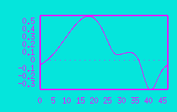
Click (N) to begin the calculation of the new adjoint. It should not take long. Click (Esc) to get to the main menu and then click (X) (Enter) to plot "V" versus t. XPP has replaced the periodic orbit with the components of the adjoint or response function. You should see something like

although there may be a phase shift. If the colors look wrong, it was probably in the food you ate. You can switch between the periodic orbit and the adjoint by clicking (U) to get to the numerics menu and then (A) to get the adjoint menu and choosing (A) or (O) for the adjoint or orbit respectively. Then with a click of (Esc) go back to the main menu and plot with the (X) click. If you want you can look at the other components of the adjoint. (Note that the "s" component is zero as the synapse has no effect on the presynaptic cell.)
We now want to compute the interaction function. This assumes that we couple two identical cells. Let X, Y, be the vector components of the two oscillators. Let the G(X,Y) be the coupling of cell Y to X. Like X, G is also a vector with components, g1,g2,... Thus, to compute the interaction function, we must tell XPP each of the components of the coupling function. XPP knows the names of the variables for the oscillator X so how do we tell it the names for Y ? The names are the same as for X but have primes attached to them. Thus if V is then name of one component in X then V' is the name of the corresponding component in Y. Thus the three components of G are:
s'*(Vsyn - V)
0
0
That is the s component of the Y oscillator influences the V component of X oscillator. All other components of G are zero.
So, assuming you have the Numerics menu on the window (if not click (U) from the main window) click on (A) to get the adjoint menu and then click on (M) to make an interaction or H function. In the command line you will be asked for the three components of the coupling. You should type in the above expressions for the three components. Then after a bit of time XPP will beep to say it is done. (On slow computers this can take a bit. It takes 2-3 seconds on the HP and about 10 on my laptop.) Click (Esc) and then (X) and type in V to plot the interaction function. XPP has replaced the first component of the orbit with the interaction function. The odd part of the interaction function appears in the second component of the orbit and the even part replaces the third component of the orbit (if there is one.) Plot "w" versus time and note that it is very close to a sine function. Plot "s" versus time and see that it is close to a cosine function plus a constant. This observation suggests that we may be able to approximate the interaction function very simply as

How do we find the coefficients? Since H is periodic, that means it has a Fourier series so we can try to get the Fourier coefficients. One standard way to get Fourier coefficients is the FFT however, that is limited to data that has 2^n points. XPP computes the Fourier coefficients the way you would by just integrating. Since we generally only want the first few, this is not really slow. Certainly, it is no slower than computing the interaction function, H. Assuming you still have the H function in the browser, get to the nUmerics menu and click on (stocHastic) and then (Fourier) to compute the Fourier coefficients of whatever is in the browser. You will be prompted for the number of modes (10 is the default and is fine for this) and for the variable. Choose V since that is the column in the browser that holds the H function. In a second or two XPP beeps and if you look in the Data Browser, you will see 10 rows of numbers. The first column is the mode (0-10 in this case), the second is the cosine coefficient and the third is the sine coefficient. If you did this correctly, you should get roughly:
0  202    0
1 -298  239
2   29  -30
3   26   1.7
 .......
As our intuition told us 90% of the power is in the first 2 terms, so by dividing by 300 (a nice round number) we get a0=.667, a1=-.98,b1=.8174 as our approximate H scaled by 1/300.
In fact, it is fun to compare the real H with the approximate.


A fixed point of this equation means that the phase-difference between the two oscillators is fixed and we say they are phaselocked. If the interaction functions are identical as for symmetrically coupled oscillators, then g is the odd part of the interaction function. This is why XPP computes the odd part of the interaction function: the zeros tell you the phase-locked solutions; those for which g has a positive slope are stable and those for which g has a negative slope are unstable
For the present case, there are two roots to the odd part. (Look at the w component of the H function -- click (nUmerics) (Adjoint) (Hfun) (Esc) (Xi vs t) w (Enter) to see it.) One of the roots is 0, or synchronous firing of the neural oscillators and the other is half a cycle a way or anti-phase. For this model synchrony is stable and anti-phase is unstable. The homework below shows other interesting behaviors.
 v'-v
0
0
What are the stable phase-locked states for this type of coupling?
Homework 3.2
Fire up the post-inhibitory rebound model
that you studied in Homework 2.4. Set
I=-1 and set Dt=.25 Find the periodic solution
for this value of current. ( Hint: It has a period of about
140.75.) Compute the adjoint or response function. Then compute the
interaction function using
Learn more about Phase Equations

 Table of Contents
 Main Menu Items
 ODE Files and Examples
 Numerics Menu
 File Menu
 Freeze Menu
 AUTO Menu
 Data Browser
 I/O and Hardcopy
 XPP Basics
 Nonlinear ODEs
 Two-dimensions
 Three-dimensions
and Beyond
 Phase Equations
 Chaos
Chaos