So far, we have looked at a scalar equation for a membrane with a single nonlinear channel. We hinted above that by letting the current vary slowly as a function of the current, we could induce oscillations in the membrane. Real membranes do this but not by directly varing the current. Rather, in addition to the fast inward calcium current, there is an additional voltage controlled outward current due to potassium. That is, the potassium current turns on with high enough voltage and hyperpolarizes the membrane. The equations for this model; the "Morris-Lecar" model are:
where

We will also track the main currents, ICa and IK. Click HERE to see the source.
Let's set up the window so we can explore this system. Time is measured in milliseconds so click (nUmerics) to get the numerics menu. Change (Dt) to .25 and change (Total) to 100 msec. Since the currents can get quite large, change (Bounds) from 100 to 1000. Click (Esc) to return to the main window. Click on (W) (W) to change the dimensions of the window:
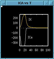
To understand this, it helps to look at the two currents. Click on (H) (C) to create another window. Click (X) and type in ICa followed by (Enter) and you will see the large negative calcium current plotted in the window. Now in the mainwindow, click (G) (A) to add another curve to the plot. A new window will appear. Type IK where it asks for the Y-axis and type in a number from 1-9 for the color (1=red, 9=violet) and then type (Ok) to accept it. ( Note: This is different than freezing a curve which keeps a permanent copy of the curve you have frozen. Adding a curve just tells XPP to plot the variables you have added at every simulation. If you change parameters or initial conditions, the added curves will change to reflect this. Frozen curves do not change.)
You will not see the new curve since XPP has not given you the best window. You can manually increase the window, or let XPP do it. Click (W) (F) to fit the window. (NOTE: This only works in versions of XPP higher than 1.6.) Otherwise just use (W) (W) and make the vertical scales from -380 to 270.
Click (T) for text and at the prompt type in "ICa" and (Enter). Using the mouse, place the text next to the big negative calcium current and click it. Repeat this for "IK." If you have done this, you will see something like:

Now we can see what excitability means. Once the voltage crosses threshold there is a large inward calcium current. After this reaches its peak causing the voltage to increase, the large outward potassium current comes into play. This is sufficient to cause the membrane to repolarize back to rest.
Homework 2.1
What is the most negative value of the calcium current and the most
positive of the potassium. (Use the Data
Viewer
(F)ind option.)
Integrate the differential equations again with a subthreshold initial
voltage, say V(0)=-20. How are the currents different from the
spiking case. (You may have to click into the small window and then
click on (R)estore to redraw the graphs.)

Click inside the big graphics window showing the voltage. Click on (H) (K) to kill all extra windows and answer (Yes). This will get rid of the little window. Now click on (U) to go into the (nUmerics) window and change the (Total) time to 250 msec and hit (Esc) to return to the main window. Click (V) (2) to get a Two-d view of the voltage and the potassium gating variable, w . A new window will appear. You must tell XPP the variables for the X and Y axes, the (optional) labels and dimensions of the window (although this can be done with the (Window) command.) We want the "X-axis" to have voltage and the "Y-axis" to have the gating variable. Fill it in as:
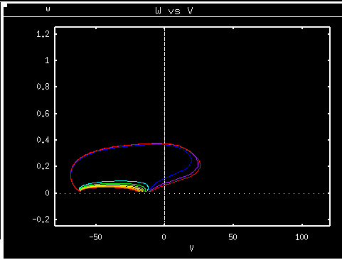
This is called a phase-plane picture and it is what the "PP" in XPP stands for. The phase-space for the Morris-Lecar model is two-dimensional and this provides a nice compact way of seeing what the solutions do as a function of time. Click (I) (N) and set V(0)=-20 and leave w as is. Note the small trajectory thet goes to the left. Now initialize V(0)=-10 and see the difference. The trajectory loops through the two-dimensional plane before returning to rest. Note that the phase-plane view shows you that the voltage increases and the gating variable slowly increases. The voltage reaches a maximum but the gating variable continues to increase reaching a maximum and then decreasing. The voltage udershoots the equilibrium before returning to rest.
Now click on (S) (M) to use the mouse to make an initial guess for a singular point or equilibrium. Click the mouse near where the two trajectories have ended. Answer (No) to the "Print Eigenvalues" question. A small circle will appear in the phase-plane that shows the position of the equilibrium. The stability window tells you you have a rest state at V=-60.89 and w=.014, that it is stable, and that the two eigenvalues are complex.
Click on (I) (M) to choose initial conditions in the phase-plane with the mouse. Click anywhere in the plane and the trajectory will be plotted. In particular, try a bunch of initial conditions near w=0 along the V-axis. Turn off the Bell by clicking (F) (B). Now click (I) (L) to get a trajectory that starts close to the initial condition. ((I) (L) means use the (Last) value of the previous trajectory as the starting point of this one.) Now click (I) (R) to do a range integration. A new window will appear. Choose V to be the variable to range over. Choose 10 Steps, with the start at -20 and the end -10. Answer yes to all three questions and click (Ok). You will see 10 colored trajectories with a clear point indicating threshold. You should see something like this:

( If this is nothing like what you see, try going through the instructions again starting at the beginning. )

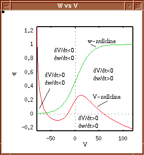
To see what is causing the threshold behavior for the neuron, it is very helpful to look at the nullclines which are curves where dV/dt=0 and dw/dt=0. The intersection of two nullclins is an equilibrium point. Click (N)(N) to make new nullclines. The "V" nullcline where V does not change is RED and the "w" nullcline, where w does not change is green. They intersect in one point, the equilibrium. Their meaning can be discerned from the figure below:

The nullclines are labeled and divide the phase-plane into 4 regions according to whether the voltage V and gating variable, w, are increasing or decreasing. THis lets you qualitatively see what happens. Use the (I) (M) command to start with initial conditions in each of the 4 regions of the phase-plane. Click on (E) to erase the screen and then on (N) (R) to restore the nullclines without having to recompute them. Now use the mouse to choose initial conditions along the line w=0 (the x-axis) near the point where the V-nullcline intersects the x-axis. Try some intial data to the left and to the right of the curve. The nullcline acts almost like a threshold.
Now set I=120 by typing (P) and then I and then the value for it. Hit (Enter) twice. If you have the parameter window open then just click on I in the window and tyoe the new value in the command line. Once again use the mouse to set the initial data. Click (I) (M) and then click the mouse in the plane. You should see a closed circle in the phase plane, a limit cycle for which both variables are periodic. Open another window and plot V as a function of t. Click (Halfwindow) (Create). Then click (Xivst) and type in V followed by (Enter). You should se a nice oscillation of the membrane potential. Click on (Xivst) and type in w and see that it oscillates as well.

We will use AUTO to find that branch of periodics as well as discover some other interesting behavior. Set I=0 and initialize V=-60.899, w=.01487. Now click (F) (A) to invoke AUTO. Now, setr up the axes by clicking on (Axes), choosing (Hi-Lo) and filling in the window as:
We are almost ready to roll!!. AUTO and XPP let us record aspects of the bifurcation curves at chosen values of parameters and periods of limit cycles. We want to get information at I=100 and, say, I=120. This is done by clicking on (Usr Period). Do this and choose 2. A window pops up. Fill in the first two entries like:
Now we can run! Click on (Run) and choose (Steady state). A thick line which is thin in the middle is drawn across the screen. The thick parts are where the steady state is stable, the thin, unstable.
How does the steady state lose stability? Click on (Grab) and move the cross-hairs until they are close to the instability. Look at the information line as you do this. You should see a symbol HB at around I=101.8 How does this compare with your estimate of the value of current which leads to instability in the homework? The symbol HB means that there is a Hopf bifurcation so we can expect to see a branch of solutions emanating from the rest state. When the cross-hair is on the HB point, click (Enter) to accept it. When you accept a point in AUTO, this sets the parameters and dependent variables to the initial condition corresponding to the point. It also gives AUTO some necessary information.
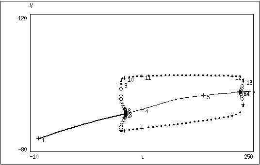
Now that we have grabbed the Hopf point, we can try to find the periodic orbit. Note: The next command may induce AUTO to loop around so once it looks like AUTO is retracing stuff it already found, click on (ABORT). So forewarned, click on (Run). Choose (Periodic) to get AUTO to trace the orbit. Stop it if it looks like its retracing! When the diagram is complete it will look like:

Filled circles represent stable periodic orbits and open circles are unstable. Notice how the unstable branch that emanates from the Hopf bifurcation bends to the left and thet the steady state solution loses stability to the right. If the direction of the bifurcating branch is opposite the direction at which stability of the main branch is lost, the branch is called subcritical and it is generally unstable. Note that there are two subcritical Hopf bifurcations; the second one is for a high current of about 220. (It is subcritical because the steady state branch loses the stability going left and the periodic branch goes right. )
Click (Grab). Using the (Tab) key, slowly click through the special points. Note the labels UZ and LP . The label UZ is a user-defined point and since we picked I=100 and I=120 , it means that I must be one of these two values. The label LP means that a limit-point or saddle node has been found. Since it occurs on a branch of periodic solutions, that means that two limit cycle orbits coalesce at this point. For this particular model, the left most limit point occurs at I = 95.72.
In many biological examples, subcritical branches from Hopf bifurcations turn around. The Morris-Lecar model, here, is such an example. Focus your attention on the region between the Hopf bifurcation and the left-most limit point, 95.72 < I < 101.8 For currents in this interval, there are 3 different possible solutions. (Imagine a vertical line drawn in this interval; it passes through three branches.) There is a stable steady state, unstable periodic, stable periodic.
If you have followed these instructions, then you will have discoverd another type of bistability between a stable fixed point and a stable periodic orbit. All initial conditions inside the unstable periodic orbit end up at the stable fixed point. All initial data outside the unstable periodic end up on the stable periodic state. The unstable periodic orbit is a threshold for repetitive firing. Create another window and plot V as a function of t for some represetative trajectories.
This concludes the tutorial on periodic, bistability, and AUTO. You can play around some more with this diagram (for example, pick some currents at the high end where there is also bistability.) When you are done, reset the bifurcation diagram to delete unwanted files from the disk: In the AUTO window, reset the diagram by clicking (File) (Reset) and answering (Yes). Exit XPP or try the next homework which is quite extensive.


 Table of Contents
 Main Menu Items
 ODE Files and Examples
 Numerics Menu
 File Menu
 Freeze Menu
 AUTO Menu
 Data Browser
 I/O and Hardcopy
 XPP Basics
 Nonlinear ODEs
 Two-dimensions
 Three-dimensions
and Beyond
 Phase Equations
 Chaos
Chaos