
If all differential equations were linear, then life would be easier but not so interesting. Most of the models that arise in real physical systems involve nonlinearities and as a consequence a much broader range of behavior is possible such as chaos and oscillations . We will continue building our simple membrane model by adding a nonlinear voltage-dependent conductance. This conductance is due to calcium. The equation is
where

This equation is already too difficult to solve analytically so one sees the advantage of numerical and qualitative techniques. (Actually, you can write the solution down in terms of an integral which you cannot evaluate except numerically!)
The ODE file for this equation in the old style is
# One fast persistent calcium channel
# Here is the equation
dv/dt=(i+gl*(vl-v)+gca*minf(v)*(vca-v))/c

#and the initial condition
V(0)=-60

# and the calcium current
aux ica=gca*minf(v)*(v-vca)

# and the parameters
param vl=-60,vca=120
param i=0,gl=2,gca=4,c=20
param v1=-1.2,v2=18

# and the functions
minf(v)=.5*(1+tanh((v-v1)/v2))
done
I have attempted to make comments which tell you what is going on. There are 2 new things here. Auxiliary quantities and User defined functions. Since functions are really important we will cover them first.
User defined functions are declared just like you would write them. They can have up to 9 arguments. Thus the function minf has 1 argument and is a squashing function. A function of 2 variables, say, f(x,y)=exp(x)*sin(y) would be written as
f(x,y)=exp(x)*sin(y)
We saw in the previous example that it was possible to add new columns to the Data Browser window. This is fine if you think of something you want to compute while in XPP. But the auxiliary declaration allows you to incorporate quantities that are not explicitly solutions to differential equations but instead some combinations of them. They are declared by starting the line with aux followed by the name of the quantity an equal sign and the definition. Now when you run this, you will be able to save the value of the calcium current and plot it as a function of time.
In the above examples, the calcium current is computed twice: once in the definition of the right-hand side and another time as an auxiliary quantity. While for this simple example, it probably doesn't matter (unless you are running on a PC with no math coprocessor) there are plenty of times when it will. If you were writing a program in C or FORTRAN you might define an intermediate quantity and use it to save on computation time. In XPP, this is done with fixed quantities that are declared by typing name=formula into the file. Fixed quantities are always evaluated before the right-hand sides are evaluated and are evaluated in the order that they are defined.
Thus, a faster version of the ode is
# One fast persistent calcium model with fixed quantities
# Here is the equation
dv/dt=(i+gl*(vl-v)-icaf)/c
#and the initial condition
V(0)=-60
# and the calcium current as a fixed quantity
icaf=gca*minf(v)*(v-vca)
# make ica available to look at
aux ica=icaf
# and the parameters
param vl=-60,vca=120
param i=0,gl=2,gca=4,c=20
param v1=-1.2,v2=18
# and the functions
minf(v)=.5*(1+tanh((v-v1)/v2))
done
NOTE XPP complains if things have the same names, thus, I
have not named the AUXILIARY and the FIXED variables the same thing.
You have now learned the essential components of an ODE file:
Consider the nonlinear pendulum
Rewrite this as a pair of first order differential equations. The frictionless energy of the system is given by:

Write an ODE file for it in the old style and then in the new style. Keep track of the energy with an auxiliary variable. Assign some positive values to all of the parameters and some random initial conditions. Answer!
Write an ODE file for the single variable continuous time Hopfield model
where

Use beta=2,theta=1,i=0,tau=1,w=1, a(0)=0 . Answer!
Now that you undestand the essentials of creating an ODE file, we will explore some more of the features of the program. Recall that we wish to explore:
where

Fire the file up by clicking on the equation. As usual the main window and the others will show up on the screen. Let's take a look at a very important set of menus:
Click (U) or on the n(U)merics part of the main menu ( i.e. type "U") and a new menu will appear.
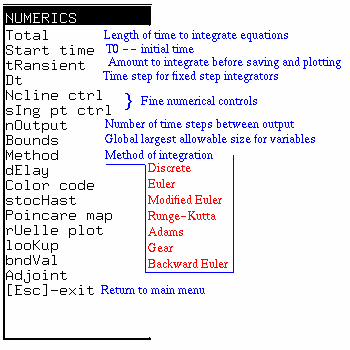
This menu is very important as it sets the parameters for all of the numerical algorithms in XPP. Details of the commands for this are found by clicking on the title of this section. I will briefly summarize the other most important commands for you. For the present example, the voltage can reach up to 120 mV. XPP attempts to prevent numerical overflow by stopping a calculation when any variable or auxiliary quantity exceeds a Bound that is set by the user. The default when XPP fires up is 100 which is less than what we would like. Set the Bound to 1000 by clicking on (B) and adding a 0 to make the global bount 1000 instead of 100. Type (Enter) when you are done. Next, we want to integrate for at least 200 msec so change the amount of time to integrate to 200. Do this by clicking on (T) for Total and changing the 20 to 200 and typing (Enter).
Now is a good time to take a look at other things in this menu. The time step for integration Dt is set by clicking on (D) and chjanging it. If Dt is negative, then the program integrates bakwards in time. The default is Dt=0.05. For this simple problem, set Dt=.2 by clicking (D), typing .2, and then (Enter). n(O)ut is important as it tells XPP how frequently you want output to plot and browse. It is set to 1 by default thus, you will get output every 0.05 msec in these examples. The t(R)ansient tells the program how long to integrate before saving and plotting the numbers. This is useful for integrating out transient effects. Start time tells the integrator what the starting time is. It is set to 0 by default and is totally irrelevant for autonoumous differential equations that do not have time explicitly in them. Finally, Method tells the program which method to use to integrate the equations. The default is Adams-Bashforth predictor corrector. The Gear method is the only presently available method in XPP which uses an adaptive step size. It will integrate stiff differential equations which are impossible to integrate using standard means. It is a very robust integrator. The other integrators are well-known and can be found in any book on numerical methods. Modified Euler is sometimes called Heun's method.
Having set the global bounds and the total integration time, return to the main menu by clicking (Esc). Set the window size by clicking (W) (W) to bring up the window box. Change it so that the X-axis goes from 0 to 200 and the y-axis from -150 to 150. Click on (Ok) or type (Tab) to enter the results. Type (I) (G) to integrate the equations. You should see a straight line across the screen. We started essentially at rest. Now type (I) (N) to manually enter new initial conditions. You will be asked for the initial voltage. Type in -20. You should see a decay to the rest state just like you saw in the linear problem. Now start with initial data of V=-10. Click (I) (N) again and then type in -10. Aha! the voltage does not decay; instead it increases to a new level of around 50 mV. This is an example of multi-stability. Nonlinear systems are often characterized by the existence of multiple stable behaviors. This cannot happen with linear differential equations (unless they are degenerate .)
Lets look at the calcium current. Create a new window by clicking (H) (C). This invokes the HalfWindow command a stupid name that is a holdover from the DOS version where the window was split in half. Grab the lower corner of the window and make it larger. Note that the window has a small square in the upper left corner that tells you it is the current plotting window. Now in the main window click (X) to choose what to plot versus time and type ICA (Enter) at the prompt. Recall that ICA is the name you gave the calcium current. You will see the calcium current plotted in the new window as a function of time. Note that it is negative and so it is an inward current. To make the voltage window the active plotting window, click the mouse inside the graph and the little square will show up on the voltage window. Make the calcium window active again. Now click the right mouse button somewhere in the picture and look at the region underneath the picture in the the main window , the info area. You should see a pair of numbers that indicate the point on the graph where you clicked. This is how you can figure out approximate values of points on your graphs. Find the time at which the calcium current is most negative. (It is about -4.7 msec.)
Make the voltage window the plotting window by clicking on it. You saw above that if you start with V=-20 then the voltage goes to an equilibrium value of about -60. If you start with V=-10 it goes to a high voltage of about 60 mV. This suggests that between -20 and -10 there is a critical value of voltage which acts as a threshold and any potential below threshold goes to the low state and above goes to the high state. Find this value, V* Then use the (S) (G) option to find the singular point or equilibrium value of voltage that is the threshold. (Answer No to both questions that XPP asks. ) Is this stable? Such a point separates the set of initial voltages into two groups: (i) those which tend to the lower voltage V < V* and (ii) those which tend to the upper voltage V > V* . These two half lines are called the domain of attraction of the lower and upper equilibria.

The program AUTO is one of the best continuation packages available and allows you to study the behavior of nonlinear dynamical systems as a function of parameters. It is part of XPP so that you can easily go between the two programs. The interface to regular AUTO involves writing lots of different FORTRAN programs, compiling them, and then running them. In this version, everything is done interactively.
To use AUTO you have to prepare your file by starting at a known steady state. When I=0 the lower steady state is -59.446. Thus start an integration with V(0)=-59.446. (I) (N) and enter the voltage at the prompt. Now you have a good guess for a steady state. It helps often to then type (I) (L) a few times - (this integrates using the end values of the previous simulation and places you even closer to a stable equilibrium.) Click (F) (A) to bring up the AUTO window. You will see a window like this:
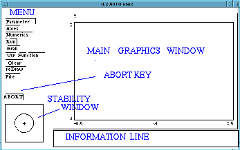
Finally, the little square with a circle in it summarizes the stability information of the solutions. All stable modes lie in the circle and unstable ones out of the circle.

Assuming you are still with me, we will now use AUTO to compute the
steady state voltage as a function of the current. (This can be done
by hand since this is a scalar differential equation. Thus, it might
seem that we are killing a  with a shotgun.
However, the basic method we use here can be easily used for other
problems. )
You should have set the initial data for the voltage to V=-59.446 and the current I=0. All other paremeters should be at their default values. (To make sure of this, go to the main XPP window and type (P). At the Parameter prompt, type the word default and the parameters will be set to their originals.)
Now click the AUTO window so that it is active. Click on the (Parameter) window and you will see a list of 5 parameters. These are the parameters that AUTO will recognize. We want to vary the current, I and since the current I is among these parameters, we don't have to change anything. Just click on (Ok).
Next, we want to set up the ranges of the diagram for plotting. Click on (Axes) and a menu will appear. We want to plot the maximum and minimum of the voltage versus the parameter, so we choose the default of HiLo. A new window will appear into which we type the necessary information. We want the "Y axis" to be the voltage, so we should type V for that entry. The main parameter is the current so change VL to I . We want the current to vary from -225 to 60 so use these values for Xmin and Xmax respectively. Finally, the voltage will range from -200 to 100 so type in these values for Ymin and Ymax respectively and then click on (Ok). Summarizing, the entries of interest should look like this:
Now, AUTO needs to know some numerical stuff. Click on (Numerics) and a window comes up with many entries. Look at the numerical description in the AUTO part of this tutorial. For now make sure of the following :
 If you did not get this, then
you should try again. Reset the diagram
by clicking (File) (Reset Diagram) and answering yes. Go back to the
main XPP window and reset the initial data to V=-59.446 and
I=0. Then repeat the above steps.
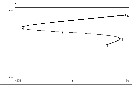
Assuming that you now have the diagram, lets traverse the diagram to see what we have computed. Click on (Grab) and a cross-hair should appear on your diagram. ( NOTE If you do not see a cross-hair then you should run XPP with the -xorfix option. That is, XPP should call xppaut -xorfix instead of just xppaut See the documentation for details.) Use the left and right arrow keys to move along the diagram. As you move, the information window at the bottom tells you stuff about the solutions such as the parameter values, the voltage value and the value of a secondary parameter. As you move along the diagram, the stability is displayed in the stability window. A quick summary of stability is seen from the diagram itself. Thick solid lines indicate stable fixed points , thin are unstable fixed points. Solid circles are stable periodic solutions and open circles are unstable periodics .
You can move through the diagram very rapidly by using the (TAB) key which only jumps to the special points. When you grab a special point, then you can do lots of other things with AUTO. Move to the point labeled 1. We will continue this curve in the negative I direction. Press the (Enter) key to accept this point. (When you (Enter) on a grabbed point, it sets all the dependent variables to the corresponding values and the relevant parameters to their values. If the point is a special point, it also tells AUTO information about the nature of the point. ) Now we have "grabbed" the starting point in our curve. AUTO has already traced out the curve in the positive I diresction. Click on the (Numerics) menu again. In the slot labeled Ds change 0.02 to -.02 so that AUTO will try to go in the other direction. Click on (Ok) to leave the numerics window and click on (Run). A branch should appear that continues until around I=-220. It is solid.
This is a complete diagram of the voltage-current relationship. There are two interesting values of the current. Traverse the diagram by clicking (Grab) and moving the crosshairs. The special point labeled 2 is denoted in the information window as LP meaning that it is a limit point. It occurs at I=36.79 A similar point at I=-210.5 is also a limit point. Both of these limit points are also called saddle-nodes or turning point bifurcations. They represent values of the parameter at which a pair of solutions comes together to form one solution. Note that the two values of current delimit the range in which there are two stable possible voltages. For -210.5 < I < 36.8 there are three steady states, two of which are stable, separated by an unstable steady state (cf. Homework 1.5 ) Thus imagine you start at the lower steady state. As you increase the current, the voltage rises until you hit I=36.8. There is a sudden increase in the potential from about -32 mV to +64mV. Now decrease the current. The potential stays high until you cross I=-210.5 at which point the potential drops precipitously. The appearance of two stable steady states gives rise to this phenomena which is known as hysteresis.
NOTE This hysteresis in the I-V curve is essential for neurons and one can see how it is then possible to get oscillatory behavior. Indeed, suppose that we make the current a varible such that when the voltage is low, the current increases and when it is high, it decreases. Then the voltage will oscillate making up and down jumps at the limit points.
AUTO (and XPP) allow you to study two parameter curves of special points. That is, we have seen that for GCA=4 there are limit points at I=36.8,-210.5. What about GCA=3 or other values of GCA. We could of course, change GCA and redo this calculation. Instead, we can fix our attention to the limit point and just compute the values of I for each value of GCA at which there is a limit point. Lets do that now. Grab special point number 2. (Click (Grab) and (Tab) to it, then hit (Enter).) Click on (Axes and choose (Two par) to do a two parameter bifurcation. We will look at the appearance of limit points for 0 < GCA < 10 and extend the current to a slightly more positive value.
Now, we want to do this for the other limit point, special point 4.
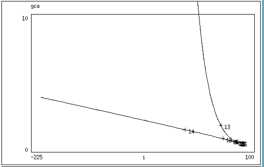
The two branches of limit points meet at a cusp point. Within the region bounded by the two curves, there are three rest states and outside of them there is one. A three-dimensional representation of this looks like:
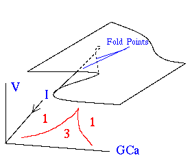
This completes the analysis of a model with a single nonlinear conductance. You should click on (File) (Reset Diagram) and click (Yes) at the prompt. This will delete all the files that AUTO creates when running a bifurcation diagram
A one-dimensional neural net is described by the following equations:


 Table of Contents
 Main Menu Items
 ODE Files and Examples
 Numerics Menu
 File Menu
 Freeze Menu
 AUTO Menu
 Data Browser
 I/O and Hardcopy
 XPP Basics
 Nonlinear ODEs
 Two-dimensions
 Three-dimensions
and Beyond
 Phase Equations
 Chaos
Chaos