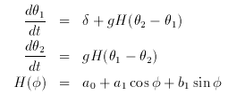

Here g is the scaled coupling strength or maximal synaptic conductance and Delta is a difference in frequency due, for example, to a different bias current to neuron 1. Fire up XPP for this model so we can look at some special plotting flags for models that lie on tori.
Notice on the menu item (phAse space). This lets us place the two variables in our maodel, X1, X2 on a circle. Click (phAse space) and then (Choose). Click (Enter) to accept the period of 2 Pi, since our model is 2 Pi-periodic. A new window appears. Use the mouse to click on both variables. Note a little X appears next to the names of the variables. (This tells XPP that each time one of these variables leaves the interval [0, 2 Pi] that it should be shifted by some multiple of 2 Pi to get it back in the interval. The plotting of such variables is "smart" enough to know not to draw extraneous lines for where the variables seem "discontinuous" because they really are not: 0 and 2 Pi are the same on a circle. ) Click (Ok) when both variables have X next to them. (Note: we could have just clicked (phAse space) (All) and that would make all plottable quantities lie on the circle, but I wanted you to see the little choice window.)
Now choose a two-dimensional view with X1, X2 as the variables and [0, 6.3] and [0, 6.3] as the window dimensions. (Click (V) (2) and fill in accordingly.)
Go into the nUmerics menu and change the total time to 200 and the time-step to Dt=.2 . Go back to the main menu and use the mouse to click in some initial data in the plane. (Use (I) (M) and position the mouse.) Trajectories all seem to end up on the diagonal line X1 = X2. This says that the oscillators always tend to synchronize since the phase-difference between them is zero. This is just what the theory told us: for this particular phase interaction function, synchrony is stable.
NOTE: If we had not defined X1, X2 to lie on the torus, we would have gotten an Out of Bounds warning after integrating the equations. Typically, phase variables monotonically increase in a nearly linear fashion with time as they cycle around their periodic phase-space. Thus the utility of using the (phAse space) option in XPP is clear.
Go back to the nUmerics menu and change Dt to -.2. This means integrate the equations backwards in time. Escape back to the main menu and click on initial conditions with the mouse. You will see that all solutions tend to a shifted diagonal line that intersects the coordinate axes at Pi. This is the other phase-locked solution and it represents a phase-shift of Pi. Since all solutions tend to it backwards in time this means it is unstable. Again as the theory told us, anti-phase solutions are unstable.
Return to the nUmerics menu and change Dt back to .2 and return to the main menu. Change the frequency difference, delta from 0 to .3 and intergate the equations with different initial conditions. Note that it still goes to a diagonal line, but this intersects the X1 axis at slightly less than 1. Thus, the phase difference between the two oscillators is about 0.9 with X1 leading X2. This is because X2 has a faster intrinsic rhythm since delta>0. Make delta negative and you will see that X2 leads X1. In either case, there is a stable phase-locked solution for this model.
We can attempt to understand this behavior a little better by reducing the equations via a map: the Poincare section. Imagine a vertical line through X1=3 for example. Looking at the phase plane, one sees that the trajectory hits this line at different values of X2. Given a value of X2 on the line, the dynamics yields a new value of X2 the next time it hits that line. The line is called a Poincare Section and the map X2(n-1) --> X2(n) is called the Poincare Map. The Poincare map always reduces the dimension of the system by one and changes the dynamics from continuous to discrete.
XPP provides a tool for studying Poincare sections. Click on (nUmerics) to get to the numerics menu and then on (Poincare) to set up the Poincare map. Choose (Section) since we are interested in when the trajectory crosses a particular value of X1 and not on maxima or minima. XPP is presently limited to looking at sections that are along the coordinate axes of the dynamic variables. (Eventually, I will make it more general.)
They are not really uniformly distributed, but seem to be denser around X2=1.5 Let's verify that now by computing a Histogram for the data.
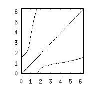
First set up the window so that it is a 2D plot with X2 on both axes: Click (View axes) (2d) and put X2 on both axes which should both be windowed between 0 and 6.3. You will see a diagonal line representing X2 vs X2 as expected. (It will not be a solid line, but, instead, a series of points.) Now, click (nUmerics) to enter the numerics menu and then click on (rUelle plot) to set negative shifts of the data. (This is named for David Ruelle who showed that dynamical sysyems could be reconstructed from time series by looking at the data plotted against a shifted version of itself. ) We will shift the X coordinate by 1 so that we will then plot X2(n) vs X2(n-1) where X2(n) is the y-coordinate and X2(n-1) is the x-coordinate. Thus, we can see if there is a reasonable looking map.
At the command-line prompt, set

with or without the diagonal line. Clearly, there is some sort of smooth function plotted here.

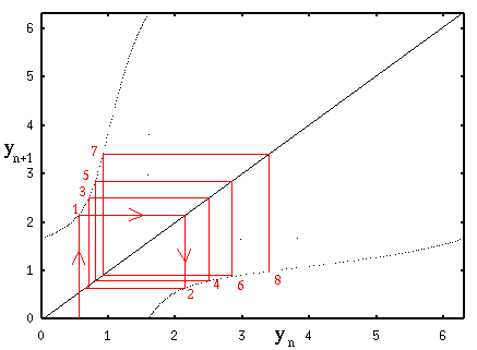
Given a starting point, you compute the new value using the map (1), then project back down by reflecting on the line y=x to get the next point (2) and so on.

This is an example of a discrete dynamical
system. The ODE file is
similar to that of an ordinary differential equation.
XPP has a method for solving this type of model.
Instead of integrating the equations, XPP iterates them. Since this
is again a model on the circle, you should invoke the (phAse space)
command followed by (All) and then accepting the default of 2
Pi. Next, change the linestyle to 0 (Click (Graphics) (Edit) 0 and
change the linestyle entry to 0.) Finally, go into the numerics menu
and change the total amount of time to, say, 1000, and change the
method of integration to (Discrete).
This tells XPP to treat this iteratively rather than as a continuous
dynamical system. (Esc) to the main menu and integrate the equations.
Plot using (Xi vs t). It looks similar to what you have already
plotted for the Poincare map. The standard map is a good
approximation for out Poincare map as long as the parameter g
in the standard map is small. If this parameter is too large,
then even with delta=0 the map becomes chaotic an interesting phenomenon that we
will look at shortly.
Homework 3.3
h(phi) = a0 + a1*cos(phi) + b1*sin(phi)+a2*sin(2*phi)First study the stable and unstable phase-locked behavior for delta=0 as you vary the amplitude of a2 letting it be both positive and negative. Then, let delta be such that phase-locking is lost. Study the Poincare map.
Note that if Y(n)=Y(n-1) then there is a fixed point for the map. Use the Ruelle plot to show there is only one fixed point.
Similarly, if Y(n)=Y(n-2) that means that there is a fixed point of the second iterate, a so called period two point. For delta=0,g=-5 use the Ruelle plot to determine how many period two points there are. ( Hint: First plot without a shift to get the diagonal line. Then plot with a shift without erasing the first line.)

 Table of Contents
 Main Menu Items
 ODE Files and Examples
 Numerics Menu
 File Menu
 Freeze Menu
 AUTO Menu
 Data Browser
 I/O and Hardcopy
 XPP Basics
 Nonlinear ODEs
 Two-dimensions
 Three-dimensions
and Beyond
 Phase Equations
 Chaos
Chaos