

Every ODE file consists of a series of lines that start with a keyword followed by numbers, names, and formulas or declare a named formula such as a differential equation or auxiliary quantity. Only the first letter of the keyword is important; e.g. the parser treats "parameter" and "punxatawney" exactly the same. The parser can understand lines up to 256 characters. You can use line continuation by adding a backslash character. The first line of the file cannot be a number (as this tells XPP that the file is in the old-style) but can be any other charcter or declaration. It is standard form to make the first line a comment which has the name of the file, but this is optional.
# comments
 option  <filename>
...
d<name>/dt=<formula>
<name>'=<formula>
...
<name>(t)=<formula>
volt  <name>=<formula>
...
<name>(t+1)=<formula>
...
<name>=<formula>
...
<name>(<x1>,<x2>,...,<xn>)=<formula>
...
init <name>=<value>,...
...
<name>(0)=<value>
...
aux <name>=<formula>
...
bdry <expression>
...
wiener <name>,...
...
parameter <name>=<value>, ...
...
number <name>=<value>
...
table <name> <filename>
...
table <name> % <npts> <xlo> <xhi> <function(t)>
...
global sign {condition} {name1=form1;...}
...
markov <name> <nstates>
{t01} {t02} ... {t0k-1}
{t10} ...
...
{tk-1,0} ...
...
# comments
...
@  <name>=<value>  ...
done
dx/dt=F(x,y,...)or
x'=F(x,y,...)Similarly, difference equations can be written as:
x(t+1)=F(x,y,...)
x(t) =  ...int{K(u,t,t')}...
x(t) =  ...int[q]{K(u,t,t')}...
x(t) =  ...int{k(t)#u}...
x(t) =  ...int[q]{k(t)#u}...
with the following meanings
zippy=f(x,t,...)Thus zippy could be used in seceral different places and yet is computed only once.
f(x,y) = x^2/(x^2+y^2)They can have up to 9 arguments.
x(0)=3
y(0)=-2
or
init x=3,y=-2Initial data are optional, XPP sets them to zero by default and they can be changed within the program.
number of values
xlo
xhi
y(xlo)
.
.
.
y(xhi)
The function form of the table require the percent symbol followed by the number of points, tlo, thi and the function of t.


XPP has many many internal parameters that you can set from within the program and four parameters that can only be set before it is run. All of these internal parameters can be set from the ``Options'' files described above However, it is often useful to put the options right into the ODE file. NOTE: Any options defined in the ODE file overide all others such as the ones in the OPTIONS file. The format for changing the options is:
@ name1=value1, name2=value2, ...where name is one of the following and value is either an integer, floating point, or string. (All names can be upper or lower case). The first four options can only be set outside the program They are:
The remaining options can be set from within the program. They are

# passive membrane model

# The parameters:
parameter c=20,gl=2,vl=-60,i=2

# the differential equation:
dv/dt=(gl*(vl-v)+i)/c

# initial data:
v(0)=0
# The initial data is not needed here as the default is 0

# tell it you are done
done
It is pretty much self-explanatory. Initial data are declared like:
name(0) = valuewhere "name" is the name of a variable which satisfies a differential equation. This is fine for one or two variable systems, but if you have many, then it is a pain to write each one on a line. Instead, you can write:
init name1=value1, name2=value2, ...Differential equations in the new format are declared as
name' = right-hand-side
# OR
dname/dt = right-hand-side
The order of most declarations in the is unimportant since the program makes two passes through the file.

# Morris-Lecar reduced model
dv/dt=(i+gl*(vl-v)+gk*w*(vk-v)+gca*minf(v)*(vca-v))/c
dw/dt=lamw(v)*(winf(v)-w)
# where
minf(v)=.5*(1+tanh((v-v1)/v2))
winf(v)=.5*(1+tanh((v-v3)/v4))
lamw(v)=phi*cosh((v-v3)/(2*v4))
#
param vk=-84,vl=-60,vca=120
param i=0,gk=8,gl=2, gca=4, c=20
param v1=-1.2,v2=18,v3=2,v4=30,phi=.04
# for type II dynamics, use v3=2,v4=30,phi=.04
# for type I dynamics, use v3=12,v4=17,phi=.06666667
v(0)=-60.899
w(0)=0.014873
# track some currents
aux Ica=gca*minf(V)*(V-Vca)
aux Ik=gk*w*(V-Vk)
done

Post-inhibitory Rebound
This model is the simplest neural oscillator. There is only one
active channel. The equations are due to Wang and Rinzel. The
equations include the activation of the fast GABA_A and slow GABA_B
synapses.
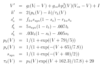
A good set of parameters is: gca=1,vk=-90,fh=2,vca=120, gl=.1,vl=-70,i=0, gsyna=0,gsynb=0,vsyna=-85,vsynb=-90,tvsyn=-40, fka=2,rka=.08. Try looking at the phase-plane with -75 < V < 20 and -.125 < h < .5. By letting the current be slightly negative, try and get this baby to oscillate. Look at the nullclines as a function of the current.
Hint Integrate it for about 200 msec with DeltaT=.1.
If you still don't think you can create the ODE file yourself, click here!

The Hodgkin-Huxley equations are the classic model for action potential propagation in the squid giant axon. They represent a patch of membrane with three channels, sodium, potassium, and a leak. The equations are:
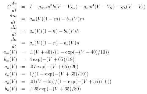
You should explore them as the current, I increases. Try to find the Hopf bifurcation. Show that there is a region where there is bistability between a periodic and fixed point. This bistability was the basis for an experiment done by Rita Gutman in the 70's.
The ODE file is:
# Hodgkin-huxley equations
dv/dt=(I - gna*h*(v-vna)*m^3-gk*(v-vk)*n^4-gl*(v-vl))/c
dm/dt= am(v)*(1-m)-bm(v)*m
dh/dt=ah(v)*(1-h)-bh(v)*h
dn/dt=an(v)*(1-n)-bn(v)*n
par vna=50,vk=-77,vl=-54.4,gna=120,gk=36,gl=.3,c=1,i=0
am(v) =  .1*(v+40)/(1-exp(-(v+40)/10))
bm(v) =  4*exp(-(v+65)/18)
ah(v) =  .07*exp(-(v+65)/20)
bh(v) =  1/(1+exp(-(v+35)/10))
an(v) =  .01*(v+55)/(1-exp(-(v+55)/10))
bn(v) =  .125*exp(-(v+65)/80)
init v=-65,m=.052,h=.596,n=.317
done
Back to the tutorial

# Morris-Lecar reduced model
dv/dt=(i+gl*(vl-v)+gk*w*(vk-v)+gca*minf(v)*(vca-v))/c
dw/dt=lamw(v)*(winf(v)-w)
ds/dt=alpha*k(v)*(1-s)-beta*s
minf(v)=.5*(1+tanh((v-v1)/v2))
winf(v)=.5*(1+tanh((v-v3)/v4))
lamw(v)=phi*cosh((v-v3)/(2*v4))
k(v)=1/(1+exp(-(v-vt)/vs))
param vk=-84,vl=-60,vca=120
param i=80,gk=8,gl=2, gca=4, c=20
param v1=-1.2,v2=18,v3=12,v4=17.4,phi=.066666667
param vsyn=120,vt=20,vs=2,alpha=1,beta=.25
# for type II dynamics, use v3=2,v4=30,phi=.04
# for type I dynamics, use v3=12,v4=17.4,phi=.06666667
v(0)=-24.22
w(0)=.305
s(0)=.056
done
Back to the salt mines ...
# phase model based on ML example
p a0=.667,delta=0,a1=-.98,b1=.8174,g=.25
h(phi)=a0+a1*cos(phi)+b1*sin(phi)
x1'=delta+g*h(x2-x1)
x2'=g*h(x1-x2)
d
This discrete dynamical system has the oldstyle format:
# standard map
y(n+1)=y+delta-g*sin(y)
par g=.35,delta=.5
done

The Lorenz equations are a three dimensional dynamical system representing turbulence in the atmosphere:
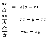
where r=27,s=10,b=8/3. The ODE file is:
# the famous Lorenz equation
init x=1,y=2
p r=27,s=10,b=2.66666
x'= s*(-x+y)
y'= r*x-y-x*z
z'=  -b*z+x*y
d

Unfolding of the triple zero
The ODE file :
# triple zero unfolding
x'=y-mu*x
y'=z-nu*x
z'=q*x*x-gamma*x
p mu=1,nu=2,gamma=1,q=2
done
The ODE file for the approximate map for this system is
#map for triple-xero
z(0)=2
par a=2.93,b=-1.44,c=1.85
z(t+1)= a+b*(z-c)^2
done
The ODE file for computing the Liapunov exponent for the map is:
# Liapunov exponent
init z=2,zp=0
aux lexp=zp/(t=1)
par a=2.93,b=-1.44,c=1.85
z(n+1)= a+b*(z-c)^2
zp(n+1)= zp+log(abs(2*b*(z-c)))
d

Other examples with some commentary
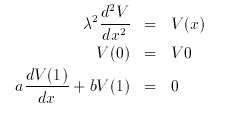
Hint Solve this equation by setting the total integration time to 1 and then using the boundary-value solver command (B) (S). Try ranging from b=0 to b=10 and plotting the results in different colors.
Since this is a second order equation and XPP can only handle first order, we write it as a system of two first order equations in the file is:
# Linear Cable Model

# define the 4 parameters, a,b,v0,lambda^2
p a=1,b=0,v0=1,lam2=1
# now do the right-hand sides
v'=vx
vx'=v/lam2

# The initial data
v(0)=1
vx(0)=0

# and finally, boundary conditions
# First we want V(0)-V0=0
b v-v0
#
# We also want aV(1)+bVX(1)=0
b a*v'+b*vx'
# Note that the primes tell XPP to evaluate at the right endpoint
d

Note that I have initialized V to be 1 which is the appropriate value to agree with the first boundary condition.

Hint Set the maximal delay to 10 by clicking (U) (E), setting it, and returning to the main menu. Then integrate the equations varying tau which is the delay. For what value of delay is the rest state unstable?
The equations are:
# delayed feedback

# declare all the parameters, initializing the delay to 3
p tau=3,b=4.8,a=4,p=-.8
# define the nonlinearity
f(x)=1/(1+exp(-x))
# define the right-hand sides; delaying x by tau
dx/dt = -x + f(a*x-b*delay(x,tau)+p)
x(0)=1
# done
d


where the Markov variable z has two states and a transition matrix dependent on x1 given by:

Hint Set the total integration time to 40, window the X-axis between 0 and 40, and add a graph of x2 along with x1. Integrate this several times to see that x2 spontaneously arises once x1 is large enough and then like all really cool mutants takes over and kills x1.
Without further ado ...
# Kepler model

# another way to do initial data
init x1=1.e-4,x2=1.e-4
p eps=.1,a=1
x1' = x1*(1-x1-x2)
x2'= z*(a*x2*(1-x1-x2)+eps*x1)
# the markov variable and its transition matrix
markov z 2
{0} {eps*x1}
{0} {0}
d

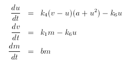
This is a normal looking model with exponential growth of the mass. However, if u decreases through 0.2, then the ``cell'' divides in half. That is the mass is set to half of its value.
Hint Set the total integration time to 800 and nOut to 10, integrate the equations, and then plot the mass versus t .
We want to flag the condition u=.2 with u decreasing through .2 so we want the sign=-1. Here it is:
# tyson
i u=.0075,v=.48,m=1
p k1=.015,k4=200,k6=2,a=.0001,b=.005
u'=  k4*(v-u)*(a+u^2) - k6*u
v'= k1*m - k6*u
m'= b*m
global -1 {u-.2} {m=.5*m}
done


Note that it is a convolution equation, so XPP can take advantage of that and speed up the problem considerably. I show you the ODE file with and without the convoltuion speed up. The closed form solution to this equation is u(t)=sin(t).
Hint Plot the solution along with the auxiliary variable, utrue to see that the solutions are the same.
The source without using the convolution speed up in the is:
# Volterra equation with actual solution
u(t) = sin(t)+.5*cos(t)-.5*t*exp(-t)-.5*exp(-t)+int{(t-t')*exp(-(t-t'))*u}
a utrue=sin(t)
d
A much faster version takes advantage of the convolution structure. The ODE file is:
# Faster version of testvol.ode
u(t)=sin(t)+.5*cos(t)-.5*t*exp(-t)-.5*exp(-t)+int{t*exp(-t)#u}
a utrue=sin(t)
done

Have a nice day!

 Table of Contents
 Main Menu Items
 ODE Files and Examples
 Numerics Menu
 File Menu
 Freeze Menu
 AUTO Menu
 Data Browser
 I/O and Hardcopy
 XPP Basics
 Nonlinear ODEs
 Two-dimensions
 Three-dimensions
and Beyond
 Phase Equations
 Chaos
Chaos